Reinforcement Learning Applied to Large Language Models
Research Essay
Table of Contents
This paper examines reinforcement learning (RL) techniques commonly applied in the fine-tuning process of large language models. The full fine-tuning process will be explained, with the focus on the commonly applied reinforcement learning methods. Additionally, possible non-RL alternatives will be mentioned as well, to provide a comprehensive overview about the advantages and challenges of RL.
About this paper
Research Essay for the course Reinforcement Learning (DLMAIRIL01), Master of Science - Artificial Intelligence at IU International University. Tutor: Dr. Janki Dodiya. Matriculation number: IU14090306.
The original LaTeX source, the bibliography, the code and the compiled PDF are available on GitLab: gitlab.com/iu-msc-ai/reinforcement_learning_dlmairil01
Introduction
This paper discusses how reinforcement learning (RL) techniques are applied to large language models (LLMs), during the fine-tuning step. Fine-tuning is a post-training step, to make the LLM more user-friendly, refine behaviors and unlock new skills. It is executed after the main training, via self-supervised learning on large amount of data (commonly via Transformer methods), is done (sometime called pre-training).12 Compare the figure below, for an exemplary training process for LLMs, which includes the pre-training and fine-tuning steps:
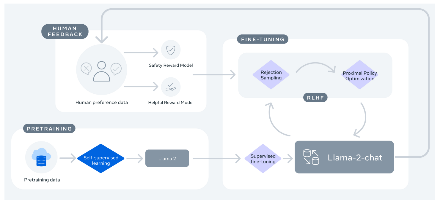
A high level overview of the fine-tuning process will be provided and the role of reinforcement learning as part of it. Then commonly applied RL methods like Proximal Policy Optimization (PPO) will be discussed in detail. Additionally, non-RL methods will be shown and discussed briefly, to show the differences compared to RL. Finally, after a brief summary, a conclusion will be drawn and an outlook on future developments will be provided.
The notation of the shown equations, from various sources, is harmonized, to make it easier for the reader to compare them and understand the differences.
Fine-tuning LLMs
With the pre-training of an LLM a so-called “base model” is created, which is usually good at next token prediction, but not good at showing the behavior we expect from LLMs nowadays, e.g. providing a well-structured answer to an input question (compare core skills in the Tülu 3 figure). Therefore, fine-tuning is applied to make the LLM more user-friendly and conversational.3 This process is called “preference alignment” and commonly done in multiple steps:
- Instruction fine-tuning
- Preference fine-tuning
- Reinforcement fine-tuning with verifiable rewards
Instruction fine-tuning is applied via supervised fine-tuning (SFT) and preference fine-tuning is done via reinforcement learning from human feedback (RLHF) or direct policy optimization (DPO), which is a non-RL technique.4 Reinforcement learning (or fine-tuning) with verifiable rewards (RLVR) is then used to improve the model on domains which do not need human feedback.5
The first two steps have been introduced by OpenAI.6 The Allen Institute for AI defined the additional third step.789 All steps are applied to build the core skills (e.g. reasoning, chatting, coding, etc.) (compare bottom left of the Tülu 3 figure) defined by the researcher.1011 Improvement on these core skills is tested during and after each step.
It is under continuous development which of these steps are executed, with how much emphasis and with which methods (e.g. possible removing supervised learning or RL steps - compare later chapters). Further the literature is not always clearly separating these steps, but always makes the distinction between supervised fine-tuning steps and fine-tuning via reinforcement learning. An example of a full training process, incl. the fine-tuning steps, was shown above. Below another example of the fine-tuning process is shown, while having the base model as a starting point. The shown process is from the Tülu 3 paper, which is a recently released LLM paper from the Allen Institute for AI (released in 2025). The architecture uses different fine-tuning steps and methods compared to the architecture shown above.
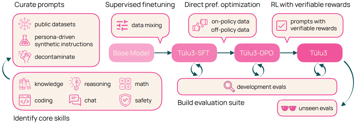
The three mentioned types of fine-tuning will be discussed in more detail now.
Supervised fine-tuning
Instruction fine-tuning, or SFT, trains the LLM on specifically selected or generated input and output samples, to refine wanted behavior, e.g. answering questions in a specific format. Technically this is not much different from the base training via semi-supervised learning, as the next token is known in the SFT case as well. The training samples are more carefully curated in this case though, to directly gear toward the defined goal(s).
The used samples (input and output pairs) are created or curated by a user called “labeler”.6 The model then, as always in supervised learning, adjusts its parameters (weights) to minimize the loss function on these samples compared to the provided output. This should already make the model more conversational and user-friendly. As in this step no RL is applied, we will not go into more detail here (compare e.g. Odds Ratio Policy Optimization for possible improvements in this step).
Preference fine-tuning
Preference fine-tuning is applied to align the LLMs output to human preferences. This can be done either via Reinforcement Learning from human feedback (RLHF) or the newer Direct Preference Optimization (DPO) approach.
Reinforcement learning from human feedback
RLHF was introduced by OpenAI in 2017, to “solve complex RL tasks without access to the reward function”, e.g. Atari games in their Gym environment.1213 Therefore it was not specifically developed for the LLM case. A complex task in a classic RL environment could be e.g. a simulated robot learning to walk.
RLHF is supposed to develop a proxy for human preferences via a reward model.14 The mentioned paper says that human feedback, from a non-expert, for 1% of the interactions of the agent with the environment, is enough to train a good agent. This is done via adding a reward predictor to the common RL setup, which is trained on human feedback. This is comparable to imitation learning and called inverse RL as well.1516 The reward from the generated reward model is then used in the same way as a reward provided from the environment in traditional RL settings (e.g. OpenAI Gym).
A schematic overview of the RLHF process is shown in the following figure. Additionally, the traditional RL process is shown for comparison:

In the RLHF paper the reward predictor is a “two layer neural network with 64 hidden units each, using leaky ReLUs”.17 The training of the predictor was done by humans by selecting the better outcome out of two provided choices, which was apparently the easiest task setup for humans that lead to good results. After training the reward predictor, the agent is trained via reinforcement learning with the reward predictor. A full pipeline with RLHF for training LLMs could look like this:
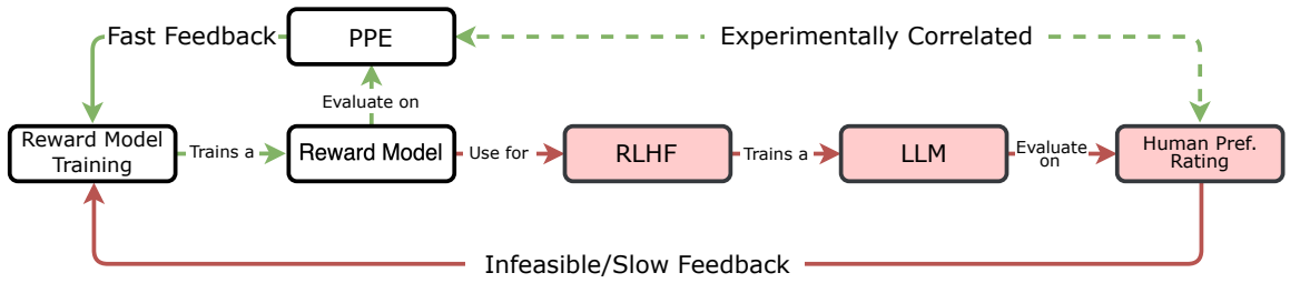
The Preference Proxy Evaluation (PPE) is an optional extra step, to evaluate the reward model, to ensure it is able to predict human preferences. This is done by comparing the reward models decision with “proxy tasks consist[ing] of a large-scale human preference and a verifiable correctness preference dataset”.1819
The LLMs output is a probability distribution over all tokens (the vocabulary of the LLM), where it usually selects the token with the highest probability from this distribution.20 This selected token could then be compared to the expected output, which is in the RL case not known though. Instead, the reward model then calculates the reward for this token and the LLM updates its parameters (weights) to maximize the expected reward. The actual optimization step in the RL process could be executed via different RL models, like Proximal Policy Optimization (PPO), which will be explained in detail later (compare Proximal Policy Optimization).
The advantage is that after training the reward predictor the pipeline can run fully automated. Training the predictor to really replicate human preferences is a challenge though. Further the LLM needs to update a lot of parameters (possibly billions) with the reward then, which is a challenge. Commonly the reward model is not used to calculate the reward after each token in the output sequence, but only the last token is assigned a reward score by the reward model.21
Direct Preference Optimization
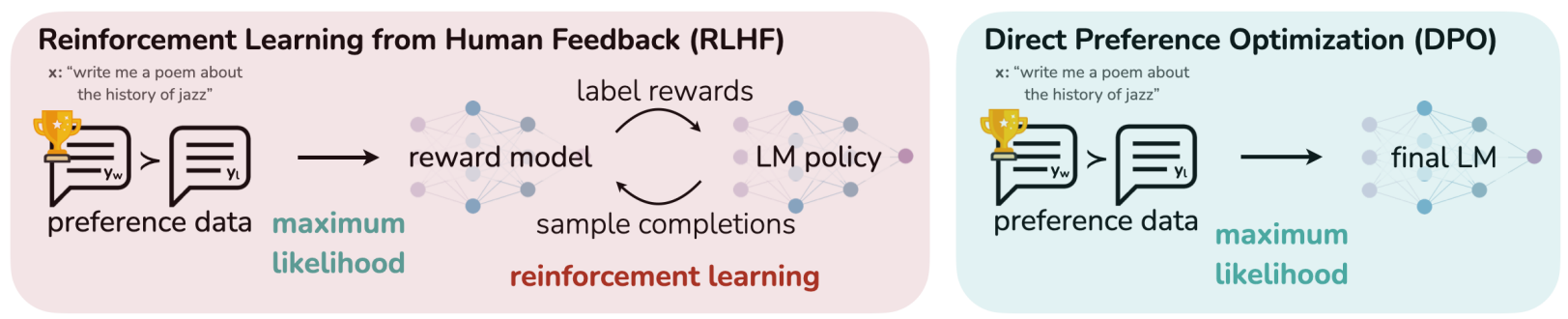
DPO is a method to train “an implicit reward model and a policy model simultaneously, without needing to use a trained reward model”.22 Therefore, it is not a RL method and “is able to bypass both fitting an explicit reward and performing RL to learn the policy using a single maximum likelihood objective”.23 We will discuss it here briefly, to show the difference to the RLHF approach.
The paper which introduced DPO in 2024, calls it a “new parameterization of the reward model in RLHF […] to solve the standard RLHF problem with only a simple classification loss”.24 The following image shows a very high level comparison between the DPO and RLHF process:
To create this implicit reward model, DPO compares the learnable policy $\pi_\theta$ and the reference policy $\pi_{ref}$ and adds a temperature parameter $\beta$. The reference policy is the initialized model from the base model, after the SFT step. The implicit reward is then defined as:2526
$$ r(x,y) = \beta\ log \frac{\pi_\theta(y|x)}{\pi_{ref}(y|x)} $$
As the reference model is the initialized model, after the SFT step, DPO limits the possible updates, comparable to the RL methods we will see later (compare Trust Region Policy Optimization and Proximal Policy Optimization).27
The loss function is defined as maximum likelihood objective and a binary cross entropy loss, which is commonly used in classification tasks and uses the previously defined implicit reward:26
$$ Loss_{DPO} = -\mathbb E_(x,y_w,y_l)\left[log\ \sigma\left(\beta\ log \frac{\pi_\theta(y_w|x)}{\pi_{ref}(y_w|x)} - \beta\ log \frac{\pi_\theta(y_l|x)}{\pi_{ref}(y_l|x)}\right)\right] $$
DPO loss function
$y_w$ is the winning output and $y_l$ the losing one. The first occurrence of the reward function should increase the likelihood of $y_w$ and the second part, connected with a minus sign, should decrease the likelihood of $y_l$. The loss function is then minimized via gradient descent, to update the parameters of the LLM.
As shown, DPO optimizes against the same goal as RLHF, without the need for a reward predictor, but still needs the human preferences.28 The optimization function used for the RL methods (e.g. PPO) was used to derive the loss function used in DPO.26
DPO can be executed via “rejection sampling”, where the LLM is trained from choices already made in the SFT stage, by curating the wanted data. The Tülu 3 paper was not able to generate significant performance gains with this method though.29
Reinforcement fine-tuning with verifiable rewards
This fine-tuning step should “boost performance on verifiable domains” and called reinforcement learning with verifiable rewards (RLVR) as well.5 RLVR can be “seen as a simplified form of existing approaches for bootstrapping LM reasoning”.7 Reasoning in LLMs is one of the mentioned desired behaviors and is technically inference-time scaling by increasing the length and quality of the Chain-of-Thought process. It is also called test-time scaling, as it “uses more computational power at inference in order to perform better at a downstream tasks [sic]”.30 Reasoning, as identified core skill, is commonly trained for in all fine-tuning steps, but as mentioned above, the authors of Tülu 3 argue for focusing on reasoning in the RLVR step.
RLVR uses “answer matching or constraint verification as a binary signal to train the model”.7 Verifiable domains are needed to have a ground truth, to calculate a reward. Besides a verifiable question answer pair (e.g. math questions, LeetCode challenges, etc.) a human preference signal can be used as well. In this case a person gets two outputs and has to select the one he prefers. Instruction following ability can be trained with this method as well.31
RLVR executes RL on LLMs. In the commonly used RL architecture the LLM is the agent, which interacts with the environment (e.g. a user) and receives a reward based on the output it generates. As always in RL, the goal of the agent is to maximize the expected reward over time. Verifiable rewards in this case means that the reward can be calculated based on a known ground truth, which is the big difference to RLHF, where the reward is based on human preference. Therefore, no reward modelling is used in the RLVR step, but the binary (scalar) signal, based on comparing the LLM output to the ground truth.
The following figure shows the schema for a RLVR setup:
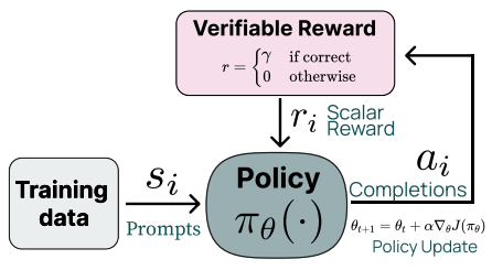
In RLVR the reward is defined as:32
$$ r(x,y) = \begin{cases} \alpha & \text{if the answer is correct} \\ 0 & \text{if the answer is wrong} \end{cases} $$
The optimization function then depends on the chosen RL method (compare Reinforcement learning methods for improving LLMs). The adjustment of the LLM works similarly as in the mentioned RLHF case. The Tülu 3 paper puts an emphasis on implementing RL/RLVR correctly, as “subtle implementation details that can significantly impact training stability”. Therefore, some implementation details are mentioned here:33
- Initialize the value model from a general reward model, which was trained in step 2
- Disable dropout, to ensure deterministic behavior
- Train with the SFT dataset (prompts and responses) over a large amount of epochs
- Ensure the model creates and End-of-Sequence (EOS) token, via a special negative reward
- Implement advantage normalization, to stabilize the training
Their findings show among other things that “RLVR can improve performance in targeted domains”, “initializing RLVR’s value function from a general RM works best” and “starting from a weaker model can converge to the same verifiable rewards”.34 Further DPO is mentioned to be less computational expensive than executing RLHF.35
Which specific RL methods can be used for RLVR and RLHF will be discussed in the next chapter in detail.
Reinforcement learning methods for improving LLMs
The currently most popular method for applying RL to fine-tune LLMs is the already mentioned Proximal Policy Optimization method. PPO is the successor to Trust Region Policy Optimization (TRPO), in regard to limiting the policy updates.36 Therefore, TRPO will be discussed first, before showing the PPO method in detail. Afterwards Group Relative Policy Optimization (GRPO) as a potential successor to PPO will be discussed.
The mentioned methods are on-policy policy methods.37 Sutton et al. defines on-policy methods as “attempt to evaluate or improve the policy that is used to make decisions” and, in distinction to this, off-policy methods as attempt to “evaluate or improve a policy different from that used to generate the data”.38 The objective of policy-based methods is “to maximize the performance of a parameterized policy”.39 All further mentioned policy based methods therefore will maximize an objective function of the following form:
$$ J(\theta) = \mathbb E_{s_0 \sim p_0} [v_{\pi_\theta}(s_0)] $$
Policy objective function
where $v$ is the value function, which is the expected return of the policy $\pi_\theta$ at state $s_0$.39
Further TRPO and PPO are policy gradient methods, which learn a “parameterized policy that can select actions without consulting a value function”.4041 These methods could still use a value function to learn the policy parameter (which is the case for PPO), but a value function is not needed for selecting the action.
A general challenge for RL methods, and especially in policy-gradient methods, is to prevent large policy updates that could destabilize the training.4243 Compared to supervised learning, where the model can correct a bad update in the next step, in RL a bad update could lead to a bad policy, which is then used to sample the next actions, which could lead to even worse updates.44 All mentioned methods have specific ways to prevent this, which will be discussed in detail.
A further challenge for RL methods is that standard gradient descent aims for the maximum possible update, which could be problematic in surfaces which “require fine control or narrow discrete actions”.42 Policy gradient methods are looking for the top of a hill (maximizing reward), instead of valleys (minimizing loss). Optimization methods (e.g. SGD or ADAM) were build for gradient descent, not ascent, “meaning they work well finding the bottom of a trough but do poorly finding the top of a ridge, especially if the ridge or hill is steep.”42
Trust Region Policy Optimization
TRPO is an on-policy policy gradient method, which was introduced in 2017, to improve reinforcement learning for simulated robots and Atari games. It was developed to improve on problems with non-trivial step sizes, by maximize a surrogate objective function. It can be applied for an “infinite-horizon discounted Markov decision process”, with finite state and action spaces.45
TRPO implements three key ideas to improve normal policy gradient methods:
- Minorize-Maximization (MM) algorithm, to maximize a lower-bound surrogate loss and therefore ensure monotonic policy improvement.
- Policy changes bound to a trust region, which is favorable to standard gradient descent methods, which are a line search method.
- Importance sampling, which is able to use samples from an old policy to calculate the policy gradient.
Minorize-Maximization
In the first step, TRPO uses a minorize-maximization algorithm, which is a method to maximize a lower-bound surrogate objective function. This is done by approximating the true objective function, which is then easier to optimize. The surrogate objective function is defined as:46
$$ \mathbb E_t \left[ \frac{\pi_\theta(a_t|s_t)}{\pi_{\theta_{old}}(a_t|s_t)} A_{\pi_{old}} \right] $$
TRPO - surrogate objective function
where $\pi_\theta(a_t|s_t)$ is the probability of taking action $a_t$ in state $s_t$ under the new policy $\pi_\theta$, $\pi_{\theta_{old}}(a_t|s_t)$ is the probability of taking action $a_t$ in state $s_t$ under the old policy $\pi_{\theta_{old}}$, and $A_{\pi_{old}}$ is the advantage function, sampled from the old policy. This is called importance sampling and is explained now.
Importance sampling
Importance sampling provides the ability to use samples from an old policy to calculate the policy gradient. As calculating the reward function for a long trajectory is expensive, the old policy is used to sample the actions and the new policy is used to calculate the reward. The result is the expected value of a function under a different probability distribution than the one used to generate the samples. As TRPO prohibits large policy updates, this error is acceptable.47 Compare $A_{\pi_{old}}$ in the surrogate objective function above.
Trust regions
Trust regions update the policy based on the Kullback–Leibler (KL) divergence between the old policy and new policy, which is a measure of how much the policy has changed. The KL divergence is used to constrain the policy update by a hyperparameter, to prevent large changes in the policy:
$$ \mathbb E_t \left[ D_{KL}(\pi_{\theta_{old}}(\cdot|s_t) || \pi_\theta(\cdot|s_t)) \right] \leq \delta $$
TRPO - KL divergence constraint
where $D_{KL}$ is the KL divergence between the old and new policy, and $\delta$ is the defined trust region. The KL divergence is a measure of how much the probability distribution (policy) changes with respect to its parameters. The trust region is a hyperparameter that controls how much the policy can change in one update. The dot in the policy ($\cdot$) represents all possible actions in state $s_t$.
TRPO “constructs the Fisher information matrix (FIM) by analytically computing the Hessian of the KL divergence, rather than using the covariance matrix of the gradients”, which is computational expensive to calculate.48 The mentioned KL constraint is approximated using the Fisher information, which therefore measures how much the probability distribution (policy) changes with respect to its parameters. Therefore, the full hessian matrix (the matrix of second derivatives of a function) is not directly needed, which would be even more computational expensive, especially in a high dimensional space, which is the case for LLMs.
To achieve the overall goal, to maximize the expected rewards, by limiting the KL divergence between the old and new policy, in combination with the minorize-maximization algorithm, and therefore staying within the trust-region, would result in following equation to be optimized:46
$$ \mathbb E_t \left[ \frac{\pi_\theta(a_t|s_t)}{\pi_{\theta_{old}}(a_t|s_t)} A_t - \beta D_{KL}(\pi_{\theta_{old}}(\cdot|s_t) || \pi_\theta(\cdot|s_t)) \right] $$
TRPO - optimization problem
where $\beta$ is a Lagrange multiplier, which is used to balance the trade-off between the two terms in the optimization problem control. The first term is the expected reward, and the second term is the KL divergence between the old and new policy.
Proximal Policy Optimization
PPO was introduced in 2017 by OpenAI and is a policy gradient method, which “optimizies a surrogate objective function using stochastic gradient ascent” via gradient descent on the policy surface.49 PPO is a so-called actor critic model, as it has a policy which is acting and a value function which is criticizing the action.
Sutton defines actor-critic methods as “methods that learn approximations to both policy and value functions”.50 The actor is the learned policy, and the critic the learned value function, which is usually a state-value function.
PPO was not specifically developed for LLMs, but according to the paper was applied to Atari games, other challenges from the OpenAI Gym and OpenAIs effort to win against professional players in Dota 2.51 These kind of tasks and LLMs have a comparable problem space though, as they just get a reward after long state-action chains. The main advantage the authors mention of PPO over TRPO is that it is easier to implement, as there is no need for hessian matrices anymore.
Clipping and bias variance trade off
Before talking about the improvements PPO offers, we need to talk about a common problem in reinforcement learning, the bias variance trade off and how PPO addresses it.
Variance is the noise in the model, which could be caused by suboptimal or wrong rewards (based on a wrong reward model). Bias is the error introduced by restricting the model (due to approximating a real world problem with a simplified model).
PPO uses clipped probability ratios, between the new and old policy. This can be considered a pessimistic estimate, to constrain policy updates and therefore reduce the variance of the model. The clipping function limits the probability ratio to a range between 1-$\epsilon$ and 1+$\epsilon$, where $\epsilon$ is a hyperparameter. This results in the policy only being able to change by a small amount, compared to the old one.52 This is a trade-off between bias and variance, as the clipping function reduces the variance, but introduces bias, as the policy can not change too much. This is comparable to the trust region in TRPO, which does it via complex mathematical calculations, while PPO does it via a simple clipping function.
The clipping function is defined as:53
$$ 1-\epsilon \leq r_\theta = \frac{\pi_\theta(a_t|s_t)}{\pi_{\theta_{old}}(a_t|s_t)} \leq 1+\epsilon $$
PPO - clipping function
where $r_\theta$ is the probability ratio and $\epsilon$ is the hyperparameter.
Optimization function
To calculate the advantage function, PPO uses a value function. The value function gives a value for each state, which ranks the state in the environment, based on the expected return (reward) from that state.
Adding everything together, the optimization function for PPO is defined as:5455
$$ \mathbb E_t \left[ min \left( \frac{\pi_\theta(a_t|s_t)}{\pi_{\theta_{old}}(a_t|s_t)} A_t, clip \left( \frac{\pi_\theta(a_t|s_t)}{\pi_{\theta_{old}}(a_t|s_t)}, 1-\epsilon, 1+\epsilon \right) A_t \right) \right] $$
PPO - optimization function
The formula uses the minimum of the probability ratio multiplied with the advantage function and the clipped probability ratio multiplied with the advantage function. This means that the policy can only change by a small amount, which introduces bias, but helps with stability and catastrophic forgetting.
Group Relative Policy Optimization
The paper introducing Group Relative Policy Optimization was published in 2024 by DeepSeek and GRPO was called as a variant of PPO.21
The main difference between GRPO and PPO is that GRPO does not use a value function and therefore should not be considered an actor-critic model anymore. Instead, GRPO is “estimating the baseline from group scores” and therefore “uses the average reward of multiple sampled outputs, produced in response to the same question, as the baseline”. This baseline is then used to calculate the advantage of the update. This reduces training resources significantly, according to the authors.
The challenge of using an average, without a value model, is that the starting model (reference model) already needs to be good enough to produce somewhat sensible output. Otherwise, the average of completely nonsensical outputs would be nonsensical as well. This works for LLMs, as a pre-trained base model exists, but would not work for classical RL problems, where the agent starts without any knowledge about the environment.
GRPO uses the following steps to update the policy (compare the GRPO figure for a visual overview):
- For each input (question) several outputs (answers) are created via the current policy.
- The reward model is used to calculate the reward for each output.
- These rewards are normalized by averaging over the group and dividing by the standard deviation of the group.
- Then the advantage is set as the final reward minus the average reward of the group, divided by the standard deviation of the group.
The formula for calculating the advantage is as follows:56
$$ A_t = \frac{R - mean(r_g)}{std(r_g)} $$
GRPO - advantage calculation without process supervision
where $R$ is the final reward of the output, $mean(r_g)$ is the mean of the group rewards and $std(r_g)$ is the standard deviation of the group rewards. The advantage is then used to update the policy (as mentioned above).
Further the group scores and advantage calculation is done just on the final action, instead of the whole trajectory.57 The authors mention that “in the LLM context, usually only the last token is assigned a reward score by the reward model, which may complicate the training of a value function that is accurate at each token”.21
For complex mathematical tasks “process supervision” is implemented, where the mentioned steps are applied to each output reasoning step of the whole output.56 So the reward is calculated for each step, but the advantage is still calculated with the mean and standard deviation of the final reward. See below:
$$ A_t = \frac{r_{j>t} - mean(r_g)}{std(r_g)} $$
GRPO - advantage calculation with process supervision
Where $r_{j>t}$ is the reward of the output at step $j$ and $t$ is the current step. Again, the advantage is then used to update the policy.
The optimization function is similar to the one PPO uses (including the clipping), but averages the objective term over the group of outputs, instead of using the value function:21
$$ \mathbb E_t \left[ \frac{1}{G} \sum_{i=1}^{G} \left( min\left( \frac{\pi_\theta(a_{i,t}|s_{i,t})}{\pi_{\theta_{old}}(a_{i,t}|s_{i,t})} A_{i,t},\ clip\left( \frac{\pi_\theta(a_{i,t}\vert_{i,t})}{\pi_{\theta_{old}}(a_{i,t}\vert_{i,t})}, 1-\epsilon, 1+\epsilon \right) A_{i,t} \right) - \beta D_{KL}(\pi_\theta || \pi_{ref}) \right) \right] $$
GRPO - optimization function
Where $G$ is the number of outputs in the group, $a_i$ is the action of the $i$-th model in the group and $D_{KL}$ is the KL divergence between the current policy and the reference policy, with $\beta$ as hyperparameter. GRPO “regularizes by directly adding the KL divergence between the trained policy and the reference policy to the loss, avoiding complicating the calculation” of the advantage.21
The following picture shows GRPO compared to PPO:
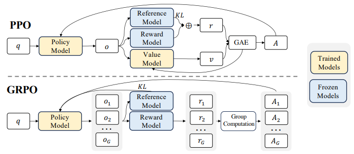
The picture shows the mentioned differences, e.g. no value model, multiple outputs and rewards per input, or applying the KL divergence to the reference policy and trained policy, shown by the arrow between them.
Removing the SFT step
With GRPO DeepSeek tried in 2025 to fine-tune a LLM without the SFT step. This model is called “R1-Zero” and was built from a base model called “V3-Base”. On top of this base model GRPO was applied, with accuracy rewards for verifiable tasks and format rewards, which made the model apply a specific output format.58 They then used a very simple prompt to get the model to reason (compare the figure below). This system prompt was added to the verifiable tasks, to generate output.5960

This template lets the model allocate more thinking time on its own. The authors show comparable results in accuracy for the fine-tuned R1-Zero model and the traditionally trained model (R1), while both started from the same base model. R1-Zero was not ready for production use though, as it had poor readability and had the tendency to switch between languages.61
Odds Ratio Policy Optimization
Odds Ratio Policy Optimization (ORPO) was introduced in 2024, by the Korea Advanced Institute of Science and Technology and is a “reference model-free monolithic odds ratio preference optimization algorithm”.8 It optimizes the odds ratio between possible actions (e.g. reduces the probability for incorrect actions).
ORPO is not a reinforcement learning approach, as it optimizes the policy directly without using a reward model, which makes it comparable to DPO (compare Direct Preference Optimization). It will be discussed here briefly anyway, to show alternatives in the fine-tuning step for LLMs and therefore helps to provide a complete picture of RL applied to LLMs. As GRPO could replace SFT in fine-tuning LLMs, ORPO could replace RL.
The following figure shows the differences between ORPO, RLHF and DPO approaches:
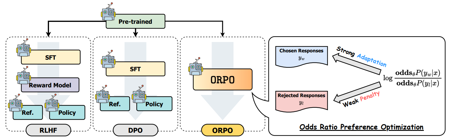
The authors of the paper argue that classical SFT via cross-entropy increases not just the likelihood of the correct token, but also output in “undesirable styles”. This is due to the cross-entropy used in SFT giving no direct penalty unwanted to output.62 That is something that ORPO tries to address, by using a preference optimization method, which is based on the odds ratio.
ORPO uses odds ratio is defined as follows:63
$$ OR_\theta(y_w, y_l) = \frac{odds_\theta(y_w|x)}{odds_\theta(y_l|x)} $$
Odds ratio
This is comparable to the DPO loss function (compare Direct Preference Optimization). The odds ratio is technically not different from the probability ratio $PR_\theta(y_w, y_l) = \frac{P_\theta(y_w|x)}{P_\theta(y_l|x)}$, but the odds ratio is more stable and less sensitive to the direct probability of the event.64
The following figure shows how ORPO rates against standard SFT and added steps applying DPO or PPO:
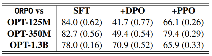
The authors show that ORPO has a win rate of mostly over 50% against the other methods in their setup, with the biggest model having the highest difference.
Comparing mentioned RL methods
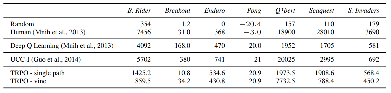
This section will compare TRPO and PPO on published and self-created results. This comparison will be done on classical RL environments and not on LLM implementations, as this offers a more direct comparison. The results mentioned in the first part have been published as part of the original publications and are not completely comparable, but should provide an intuition about the performance and performance increases of the different methods. For GRPO, as it was specifically developed for LLMs, unfortunately performance results for common RL environments are not provided, as the paper just shows the performance of the trained LLM to other LLMs. Therefore, GRPO is omitted here.
The first figure shows the performance of TRPO against Deep Q-Learning, Monte-Carlo Tree Search with supervised training (UCC-I) and a human and random policy as baseline.
The PPO paper does not show a direct comparison to TRPO unfortunately, but provides data for the same games TRPO was tested on. Unfortunately the TRPO paper does not publish all hyperparameters used for training. Therefore, the results can not be compared one to one and are therefore not shown in the same table.
| Policy | BeamRider | Breakout | Enduro | Pong | Qbert | Seaquest | Space Invaders |
|---|---|---|---|---|---|---|---|
| A2C | 3031.7 | 303 | 0 | 19.7 | 10065.7 | 1714.3 | 744.5 |
| ACER | 3863.3 | 456.4 | 0 | 20.7 | 15316.6 | 1739.5 | 1213.9 |
| PPO | 1590 | 274.8 | 758.3 | 20.7 | 14293.3 | 1204.5 | 942.5 |
PPO results - source: Schulman et al., 2017, p. 12
Assuming the tests have been conducted with the standard environments, comparing the provided results show that PPO is better in most cases (besides Pong and partly Seaquest), by mostly a wide margin.
Own performance tests
To execute a validity check for the mentioned comparison of results, and for an independent check for performance of the methods, I have implemented a small test setup, via CleanRL. CleanRL is a deep reinforcement learning library, which provides “high-quality single-file implementation with research-friendly features”.65 This setup uses classical RL environments, like the OpenAI Gym.
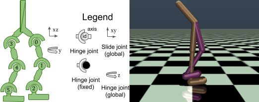
In this setup I compared TRPO and PPO for the “Walker2d-v4” environment, which is a common test environment for RL algorithms. The Walker2d-v4 environment is a 2D simulation of a bipedal walker, which has to learn to walk. The goal is to maximize the sum of rewards, which is given for each step taken and for the distance traveled.66
The setup uses the provided policy files from CleanRL and can be run via the following commands, after using the provided setup guide:6768
python cleanrl/ppo_continuous_action.py \
    --seed 1 \
    --env-id Walker2d-v4 \
    --total-timesteps 50000

python cleanrl/trpo_continuous_action.py \
    --seed 1 \
    --env-id Walker2d-v4 \
    --total-timesteps 50000
Run CleanRL policies
The mentioned policies were run for 50.000 steps and the average and maximum reward and episode length are shown below. The average values are lower for PPO, as it took the PPO policy longer to learn the task (compare the CleanRL results figure), the PPO policy ended up with a better model though.
| Policy | Avg. reward | Max. reward | Avg. length | Max. length |
|---|---|---|---|---|
| TRPO | 134.07 | 443.15 | 102.59 | 372 |
| PPO | 95.10 | 736.55 | 88.69 | 669 |
CleanRL results - TRPO vs PPO
The following figure shows steps per seconds (SPS), the explained variance, value loss and the episodic length and reward. TRPO is shown in orange, PPO in blue and all charts are on a logarithmic scale and with a smoothing factor of 0.6 (original values are grayed out).69 TRPO was able to create a good policy faster (compare episodic length and reward), but the PPO policy was able to learn a better policy in the end. Further PPO was less compute intensive (compare SPS).
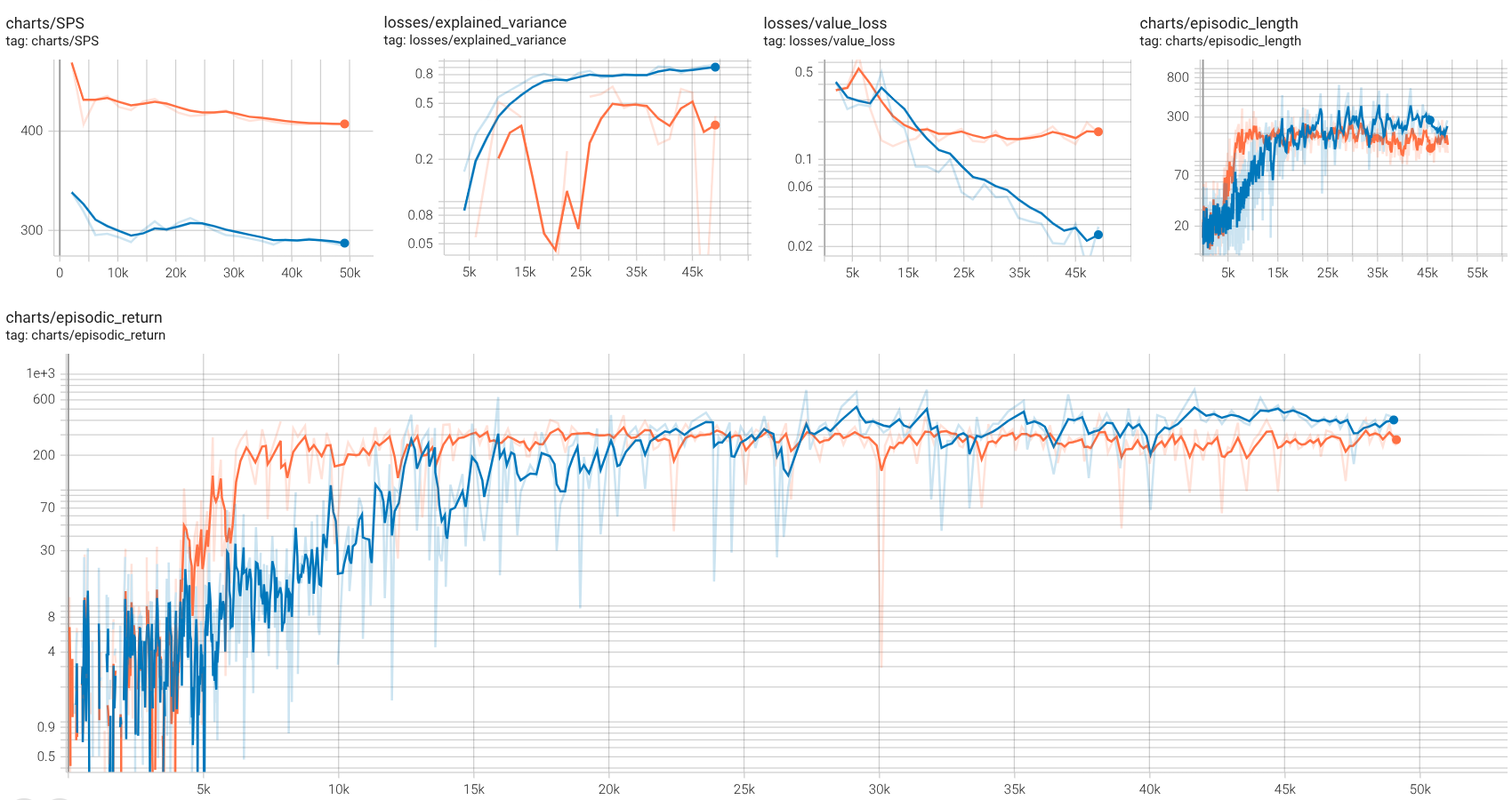
These tests confirmed the results shown earlier.
Summary and outlook
This paper showed the steps which are commonly executed in fine-tuning LLMs and how reinforcement learning methods have a key role in this process. Further the improvements in RL methods over time were shown, in regard to easier RL methods (e.g. via PPO) and the emerging possibility to remove needed fine-tuning stages (e.g. removing the SFT stage, training the mentioned R1-Zero model via GRPO).
It is interesting to see that each iteration of the RL methods published reduced complexity. PPO being a simpler algorithm then TRPO and DeepSeek, as a new player in the LLM scene, surprised with GRPO, a policy which simplified PPO even more.
Fine-tuning LLMs is a very active field of study, with especially the RL methods (e.g. TRPO and PPO) having a very large amount of citations on Google Scholar. This could be due to TRPO and PPO being older methods and being applied not just to LLMs though. The following list shows the number of citations for the mentioned papers (as of 19.05.2025) and shows the “Attention is all you need” paper, which introduced the Transformer model, a cornerstone of modern LLMs, as a baseline. The order is based on the order the publications have been mentioned in this paper:
- RLHF (2022): 14.249 citations
- DPO (2023): 3.417 citations
- TRPO (2015): 9.735 citations
- PPO (2017): 26.073 citations
- GRPO (2024): 583 citations
- ORPO (2024): 215 citations
- Attention is all you need (2017): 180.523 citations
Reinforcement learning could become the only step needed for fine-tuning LLMs (compare Removing the SFT step). Further RL could improve LLMs in areas where the semi-supervised training is not able to build a good model and even SFT would need a larger amount of highly specialized examples. Another advantage of RL is that it can run over many epochs, after a reward model is trained or especially on domains with verifiable output. For non-verifiable domains the challenge is to build a reward model that really reflects human preference though. Further RL is more complex to implement and needs more compute power than supervised learning.
There is active research in building and improving supervised learning methods, to reduce the need for reinforcement learning (compare Direct Preference Optimization and Odds Ratio Policy Optimization). RL was the starting point for fine-tuning LLMs, as it was challenging to build the same feedback mechanism back into the LLM via supervised learning and therefore not possible to build a loss function to optimize against. This did change with DPO and ORPO.
Further RL methods are commonly complicated to implement and implementation details could lead to different results.33 Therefore, easier methods are preferred in the RL community. In the Tülu 3 paper the authors mentioned even with PPO the need for “meticulous monitoring and intervention” during RL training.70
Personally I would expect DPO and RLVR methods to be a preferred combination in the future. But as already some powerful reward predictors seem to exist (e.g. OpenAI using theirs successfully for multiple different models), we may see further improvements in this field as well.
Appendix
Link to the Git repository: gitlab.com/iu-msc-ai/reinforcement_learning_dlmairil01.
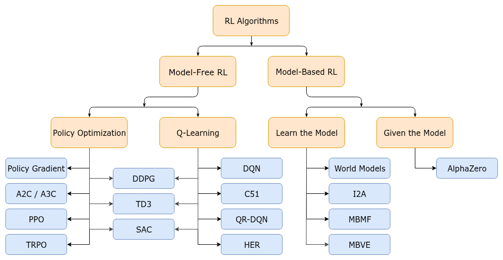
List of RL algorithms
References
Lambert, Nathan; Morrison, Jacob; Pyatkin, Valentina; Huang, Shengyi; Ivison, Hamish; Brahman, Faeze; Miranda, Lester James V.; Liu, Alisa; Dziri, Nouha; Lyu, Shane; Gu, Yuling; Malik, Saumya; Graf, Victoria; Hwang, Jena D.; Yang, Jiangjiang; Le Bras, Ronan; Tafjord, Oyvind; Wilhelm, Chris; Soldaini, Luca; Smith, Noah A.; Wang, Yizhong; Dasigi, Pradeep; Hajishirzi, Hannaneh - Tulu 3: Pushing Frontiers in Open Language Model Post-Training, 2025, p. 1. https://arxiv.org/abs/2411.15124 ↩︎
Lambert, Nathan - Reinforcement Learning from Human Feedback, 2025, p. 5, 85. https://arxiv.org/abs/2504.12501 ↩︎
DeepSeek reported that a base model with limited fine-tuning still had the tendency to switch between languages and provided poorly readable output. Compare DeepSeek-AI et al., 2025, p. 9. ↩︎
Lambert, Nathan et al. - Tulu 3: Pushing Frontiers in Open Language Model Post-Training, 2025, p. 10. https://arxiv.org/abs/2411.15124 ↩︎
Lambert, Nathan - Reinforcement Learning from Human Feedback, 2025, p. 5. https://arxiv.org/abs/2504.12501 ↩︎ ↩︎
Ouyang, Long; Wu, Jeff; Jiang, Xu; Almeida, Diogo; Wainwright, Carroll L.; Mishkin, Pamela; Zhang, Chong; Agarwal, Sandhini; Slama, Katarina; Ray, Alex; Schulman, John; Hilton, Jacob; Kelton, Fraser; Miller, Luke; Simens, Maddie; Askell, Amanda; Welinder, Peter; Christiano, Paul; Leike, Jan; Lowe, Ryan - Training language models to follow instructions with human feedback, 2022, p. 3. https://arxiv.org/abs/2203.02155 ↩︎ ↩︎
Lambert, Nathan et al. - Tulu 3: Pushing Frontiers in Open Language Model Post-Training, 2025, p. 30. https://arxiv.org/abs/2411.15124 ↩︎ ↩︎ ↩︎
Hong, Jiwoo; Lee, Noah; Thorne, James - ORPO: Monolithic Preference Optimization without Reference Model, 2024, p. 1. https://arxiv.org/abs/2403.07691 ↩︎ ↩︎
Lambert, Nathan et al. - Tulu 3: Pushing Frontiers in Open Language Model Post-Training, 2025, p. 9. https://arxiv.org/abs/2411.15124 ↩︎
Lambert, Nathan et al. - Tulu 3: Pushing Frontiers in Open Language Model Post-Training, 2025, p. 5. https://arxiv.org/abs/2411.15124 ↩︎
Touvron, Hugo; Martin, Louis; Stone, Kevin; Albert, Peter; Almahairi, Amjad; Babaei, Yasmine; et al. - Llama 2: Open Foundation and Fine-Tuned Chat Models, 2023, p. 36. https://arxiv.org/abs/2307.09288 ↩︎
OpenAI handed over the Gym environment to the Farama Foundation in 2022. As it is still common in the RL community to call it OpenAI Gym / Gymnasium, this will be done in this paper as well. Compare The Farama Foundation - Announcing The Farama Foundation. https://farama.org/Announcing-The-Farama-Foundation ↩︎
Christiano, Paul; Leike, Jan; Brown, Tom B.; Martic, Miljan; Legg, Shane; Amodei, Dario - Deep reinforcement learning from human preferences, 2023, p. 1. https://arxiv.org/abs/1706.03741 ↩︎
Wang, Binghai; Zheng, Rui; Chen, Lu; Liu, Yan; Dou, Shihan; Huang, Caishuang; Shen, Wei; Jin, Senjie; Zhou, Enyu; Shi, Chenyu; et al. - Secrets of RLHF in Large Language Models Part II: Reward Modeling, 2024, p. 1. https://arxiv.org/abs/2401.06080 ↩︎
Morales, Miguel - Grokking Deep Reinforcement Learning, Manning Publications, 2020, p. 171. ↩︎
Arora, Saurabh; Doshi, Prashant - A Survey of Inverse Reinforcement Learning: Challenges, Methods and Progress, 2020, p. 3. https://arxiv.org/abs/1806.06877 ↩︎
Christiano, Paul et al. - Deep reinforcement learning from human preferences, 2023, p. 14. https://arxiv.org/abs/1706.03741 ↩︎
This could already be considered a step in the direction of RLVR (compare Reinforcement fine-tuning with verifiable rewards). ↩︎
Frick, Evan; Li, Tianle; Chen, Connor; Chiang, Wei-Lin; Angelopoulos, Anastasios N.; Jiao, Jiantao; Zhu, Banghua; Gonzalez, Joseph E.; Stoica, Ion - How to Evaluate Reward Models for RLHF, 2024, p. 1-2. https://arxiv.org/abs/2410.14872 ↩︎
An LLM can be configured via a setting called temperature. This could add more randomness to the output, by instructing the LLM to not always use the token with the highest probability. ↩︎
Shao, Zhihong et al. - DeepSeekMath: Pushing the Limits of Mathematical Reasoning in Open Language Models, 2024, p. 13. https://arxiv.org/abs/2402.03300 ↩︎ ↩︎ ↩︎ ↩︎ ↩︎
Lambert, Nathan et al. - Tulu 3: Pushing Frontiers in Open Language Model Post-Training, 2025, p. 21. https://arxiv.org/abs/2411.15124 ↩︎
Rafailov, Rafael et al. - Direct Preference Optimization: Your Language Model is Secretly a Reward Model, 2024, p. 5. https://arxiv.org/abs/2305.18290 ↩︎
Rafailov, Rafael; Sharma, Archit; Mitchell, Eric; Ermon, Stefano; Manning, Christopher D.; Finn, Chelsea - Direct Preference Optimization: Your Language Model is Secretly a Reward Model, 2024, p. 1. https://arxiv.org/abs/2305.18290 ↩︎
The formula displayed in the paper adds a partition function $+ \beta\ log Z(x)$ to normalize the reward. This part is omitted here, as this cancels out in further optimizations later anyway. ↩︎
Rafailov, Rafael et al. - Direct Preference Optimization: Your Language Model is Secretly a Reward Model, 2024, p. 4. https://arxiv.org/abs/2305.18290 ↩︎ ↩︎ ↩︎
In all cases when a reference model is mentioned, there can be a snapshot of the further trained model replacing the initial reference model in the training process. This is a deliberate choice by the researchers then and the replacement model should be very stable again. ↩︎
In the beginning it was intuitively hard to understand why DPO would show the same or even better performance then RLHF (compare Rafailov et al., 2024, p. 1), without the reward predictor. As with a trained reward predictor the pipeline can be executed on many more samples after training it. But the same amount of human preferences and therefore information provided by humans is used in both methods. It is just applied in different ways. ↩︎
Lambert, Nathan et al. - Tulu 3: Pushing Frontiers in Open Language Model Post-Training, 2025, p. 48. https://arxiv.org/abs/2411.15124 ↩︎
Lambert, Nathan - Reinforcement Learning from Human Feedback, 2025, p. 88. https://arxiv.org/abs/2504.12501 ↩︎
Zhou, Jeffrey; Lu, Tianjian; Mishra, Swaroop; Brahma, Siddhartha; Basu, Sujoy; Luan, Yi; Zhou, Denny; Hou, Le - Instruction-Following Evaluation for Large Language Models, 2023, p. 1. https://arxiv.org/abs/2311.07911 ↩︎
Lambert, Nathan et al. - Tulu 3: Pushing Frontiers in Open Language Model Post-Training, 2025, p. 31. https://arxiv.org/abs/2411.15124 ↩︎
Lambert, Nathan et al. - Tulu 3: Pushing Frontiers in Open Language Model Post-Training, 2025, p. 32. https://arxiv.org/abs/2411.15124 ↩︎ ↩︎
Lambert, Nathan et al. - Tulu 3: Pushing Frontiers in Open Language Model Post-Training, 2025, p. 33-34. https://arxiv.org/abs/2411.15124 ↩︎
Lambert, Nathan et al. - Tulu 3: Pushing Frontiers in Open Language Model Post-Training, 2025, p. 29. https://arxiv.org/abs/2411.15124 ↩︎
Besides the limited policy updates PPO shares a lot of the underlying architecture with A2C. Compare Morales, 2020, p. 398. ↩︎
A general non-comprehensive list of RL policies published by OpenAI is shown in the appendix (compare List of RL algorithms). ↩︎
Sutton, Richard S.; Barto, Andrew G. - Reinforcement Learning: An Introduction, The MIT Press, 2018, p. 100. ↩︎
Morales, Miguel - Grokking Deep Reinforcement Learning, Manning Publications, 2020, p. 341. ↩︎ ↩︎
Non policy gradient method would be action-value methods, which policies would not exist without the action-value estimates. An example would be Q-learning. ↩︎
Sutton, Richard S.; Barto, Andrew G. - Reinforcement Learning: An Introduction, The MIT Press, 2018, p. 321. ↩︎
Lanham, Micheal - Hands-On Reinforcement Learning for Games, Packt Publishing, 2020, p. 202. ↩︎ ↩︎ ↩︎
Morales, Miguel - Grokking Deep Reinforcement Learning, Manning Publications, 2020, p. 403. ↩︎
van Heeswijk, W. J. A. - Natural Policy Gradients In Reinforcement Learning Explained, 2022, p. 2. https://arxiv.org/abs/2209.01820 ↩︎
Schulman, John; Levine, Sergey; Moritz, Philipp; Jordan, Michael I.; Abbeel, Pieter - Trust Region Policy Optimization, 2017, p. 1. https://arxiv.org/abs/1502.05477 ↩︎
Schulman, John et al. - Trust Region Policy Optimization, 2017, p. 4. https://arxiv.org/abs/1502.05477 ↩︎ ↩︎
Morales, Miguel - Grokking Deep Reinforcement Learning, Manning Publications, 2020, p. 337. ↩︎
Schulman, John et al. - Trust Region Policy Optimization, 2017, p. 5. https://arxiv.org/abs/1502.05477 ↩︎
Schulman, John; Wolski, Filip; Dhariwal, Prafulla; Radford, Alec; Klimov, Oleg - Proximal Policy Optimization Algorithms, 2017, p. 1. https://arxiv.org/abs/1707.06347 ↩︎
Sutton, Richard S.; Barto, Andrew G. - Reinforcement Learning: An Introduction, The MIT Press, 2018, p. 331. ↩︎
OpenAI; Berner, Christopher; Brockman, Greg; Chan, Brooke; Cheung, Vicki; Dębiak, Przemysław; Dennison, Christy; Farhi, David; et al. - Dota 2 with Large Scale Deep Reinforcement Learning, 2019, p. 5. https://arxiv.org/abs/1912.06680 ↩︎
Schulman, John et al. - Proximal Policy Optimization Algorithms, 2017, p. 1-3. https://arxiv.org/abs/1707.06347 ↩︎
Schulman, John et al. - Proximal Policy Optimization Algorithms, 2017, p. 3. https://arxiv.org/abs/1707.06347 ↩︎
The paper shows the probability ratio as $r_t(\theta)$ (compare the clipping function). Here the probability ratio is shown in detail, to align the equation to the others. ↩︎
Schulman, John et al. - Proximal Policy Optimization Algorithms, 2017, p. 2-4. https://arxiv.org/abs/1707.06347 ↩︎
Shao, Zhihong et al. - DeepSeekMath: Pushing the Limits of Mathematical Reasoning in Open Language Models, 2024, p. 14. https://arxiv.org/abs/2402.03300 ↩︎ ↩︎
Shao, Zhihong; Wang, Peiyi; Zhu, Qihao; Xu, Runxin; Song, Junxiao; Bi, Xiao; Zhang, Haowei; Zhang, Mingchuan; Li, Y. K.; Wu, Y.; Guo, Daya - DeepSeekMath: Pushing the Limits of Mathematical Reasoning in Open Language Models, 2024, p. 3. https://arxiv.org/abs/2402.03300 ↩︎
The output had to be enclosed by
<think>and</think>tags whenever the model was reasoning. ↩︎This confirms the earlier mentioned statement from the Tülu paper, that reasoning is build mainly by the RLVR setp (compare Reinforcement fine-tuning with verifiable rewards). ↩︎
DeepSeek-AI; Guo, Daya; Yang, Dejian; Zhang, Haowei; Song, Junxiao; Zhang, Ruoyu; Xu, Runxin; Zhu, Qihao; Ma, Shirong; Wang, Peiyi; et al. - DeepSeek-R1: Incentivizing Reasoning Capability in LLMs via Reinforcement Learning, 2025, p. 3-6. https://arxiv.org/abs/2501.12948 ↩︎
DeepSeek-AI et al. - DeepSeek-R1: Incentivizing Reasoning Capability in LLMs via Reinforcement Learning, 2025, p. 8-9. https://arxiv.org/abs/2501.12948 ↩︎
Hong, Jiwoo; Lee, Noah; Thorne, James - ORPO: Monolithic Preference Optimization without Reference Model, 2024, p. 2. https://arxiv.org/abs/2403.07691 ↩︎
Hong, Jiwoo; Lee, Noah; Thorne, James - ORPO: Monolithic Preference Optimization without Reference Model, 2024, p. 4. https://arxiv.org/abs/2403.07691 ↩︎
Hong, Jiwoo; Lee, Noah; Thorne, James - ORPO: Monolithic Preference Optimization without Reference Model, 2024, p. 8. https://arxiv.org/abs/2403.07691 ↩︎
Huang, Shengyi; Dossa, Rousslan Fernand Julien; Ye, Chang; Braga, Jeff; Chakraborty, Dipam; Mehta, Kinal; Araújo, João G.M. - CleanRL: High-quality Single-file Implementations of Deep Reinforcement Learning Algorithms, Journal of Machine Learning Research 23(274), 2022, p. 1-18. http://jmlr.org/papers/v23/21-1342.html ↩︎
More information to the selected environment can be found here: Gymnasium Documentation - Walker2D ↩︎
CleanRL installation guide: CleanRL - Installation ↩︎
The TRPO policy is still in a pending pull request and not available in the current version of CleanRL. The used code can be found here: github.com. ↩︎
This was run on a Dell XPS 13 with an Intel Core Ultra 7 155H CPU and 64GB RAM. The only metric that this should influence is SPS though. ↩︎
Lambert, Nathan et al. - Tulu 3: Pushing Frontiers in Open Language Model Post-Training, 2025, p. 46. https://arxiv.org/abs/2411.15124 ↩︎