Transformer-based ORL Applied to Chess - Part 3: Baseline and Base UDRL Results
Master Thesis, Part 3: Training metrics and the results for 1_TEO, 2_UDRL-eval, 3_UDRL-material and 4_UDRL-eval-legal_input
Table of Contents
This section presents the results of the conducted experiments. First, the training metrics are shown and discussed, followed by the evaluation results of each individual model with regard to playing strength and decision-making process. This third part covers the Chess-Transformer baseline and the base Upside Down Reinforcement Learning models - including the finding that a reward target set at inference time steers the playing strength of the model within a single game.
About this paper
Master Thesis for the Master of Science - Artificial Intelligence at IU International University.
The original LaTeX source, the bibliography, the full code, the data preparation and the compiled PDF are available on GitLab: gitlab.com/iu-msc-ai/transformer-based-offline-reinforcement-learning-applied-to-chess
This is part 3 of 4:
- Foundations
- Experimental setup
- Results - Chess-Transformer baseline and base UDRL (this part)
- Results - reward targets, manipulation and conclusion
Training metrics
All models were trained on the mentioned 9 million moves for 13 epochs, which did result ~57.000 steps due to the mentioned batch size and update frequency (compare hyperparameters). The training was always stopped after 13 epochs, as the improvements for all models stagnated by then (compare training plots below). All models have been trained on a single NVIDIA RTX 5090 GPU with 32 GB of memory. Training time for a single model was around six hours, depending on other specifications of the VM instance used for the training.1 The training curves with regard to training and validation loss and accuracy are comparable for almost all models and even comparable to the training of the original Chess-Transformer encoder model, which is shown additionally in the table and plot below.2 The final values are shown in the table and the trajectory is shown in the plots below. Plots for individual models are shown in the appendix of part 4.
| Model name | Train. Loss | Val. Loss | Train. Top-1 Accuracy | Val. Top-1 Accuracy |
|---|---|---|---|---|
| CT - original training data | 2,88 | 2,017 | 0,418 | 0,407 |
| 1_TEO | 2,486 | 2,730 | 0,537 | 0,467 |
| 2_UDRL-eval | 2,398 | 2,700 | 0,561 | 0,476 |
| 3_UDRL-material | 2,305 | 2,518 | 0,607 | 0,528 |
| 4_UDRL-eval-legal_input | 2,223 | 2,540 | 0,637 | 0,535 |
| 5_UDRL-rtg3_eval | 2,429 | 2,718 | 0,539 | 0,469 |
| 5b_UDRL-rtg5_eval | 2,394 | 2,801 | 0,561 | 0,450 |
| 6_UDRL-rtg3_material | 2,445 | 2,699 | 0,562 | 0,484 |
| 6b_UDRL-rtg5_material | 2,766 | 3,041 | 0,477 | 0,392 |
| 7_DT-eval | 4,459 | 4,426 | 0,115 | 0,109 |
| 8_UDRL-eval-manipulated_reward | 2,241 | 2,468 | 0,641 | 0,553 |
| 9_UDRL-eval-hidden_action | 2,276 | 2,517 | 0,621 | 0,535 |
| 10_TEO-Elo_signal | 2,440 | 2,742 | 0,549 | 0,464 |
Training metrics overview - source: own depiction
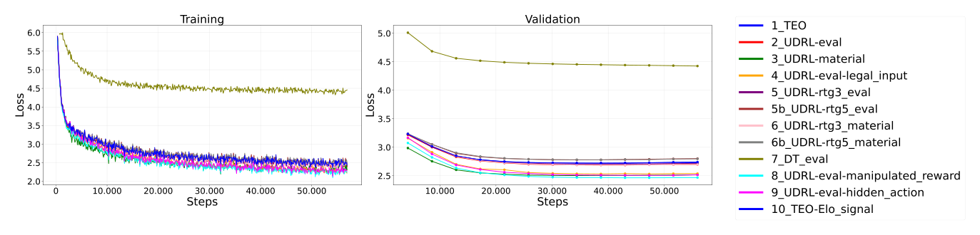
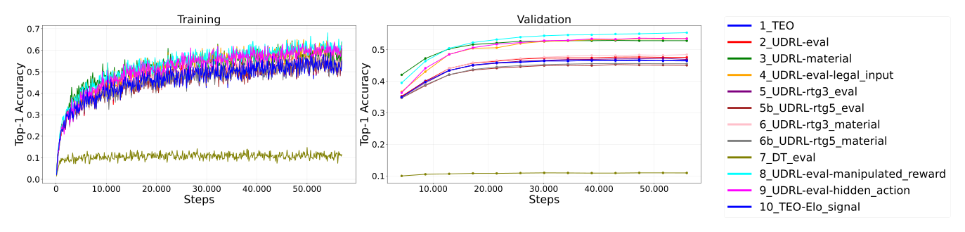
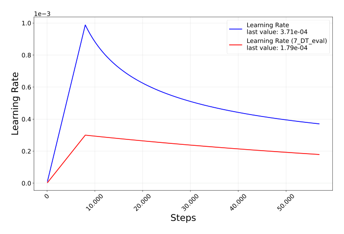
The most noticeable result in the shown training logs is the higher loss and lower accuracy of model 7_DT-eval. This will be discussed later in detail. But it can already be said that the Decision Transformer (DT) architecture does not appear well-suited for the chess domain in this setup. This model was trained with a different learning rate schedule, otherwise the training setup would not have produced any learning at all.
Further a slightly lower loss and higher accuracy for the models 3_UDRL-material, 4_UDRL-eval-legal_input, 8_UDRL-eval-manipulated_reward and 9_UDRL-eval-hidden_action is visible. This indicates that these models were able to learn better representations of the data. This does not necessarily translate to higher playing strength, which is evaluated later. Especially model 8 and 9 have not been built to analyze the playing strength, but are very comparable to model 2_UDRL-eval, just with manipulated input data for two actions.
Besides this the general training curves are comparable to the original Chess-Transformer training, indicating that the models were able to learn from the data in a similar manner. These training results are in the same ranges as the models mentioned earlier (compare Transformer architecture).
Next the individual models are evaluated in the mentioned dimensions, e.g. relative playing strength of the models, attention, logits and if necessary on further details specific to the model, to answer the research questions.
Chess-Transformer (1_TEO)
To get a starting point, the encoder-only setup of the mentioned Chess-Transformer project was trained on the preprocessed dataset. The resulting model played 500 games against Stockfish on level 2, 3 and 4. The wins, draws and losses are visualized below.
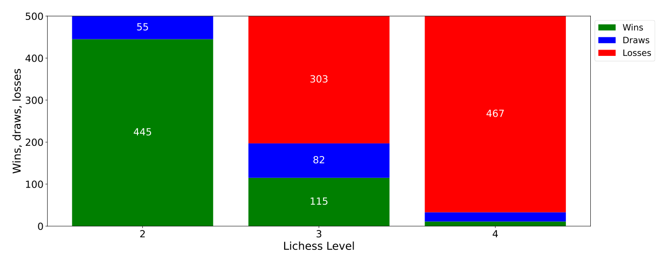
This plot shows a strong difference in playing strength between the levels. To assess statistical significance the results were tested via the mentioned Fisher’s exact test for 500 games per level. The results are shown in the table below.
| Level A | A: Wins / Losses / Draws | Level B | B: Wins / Losses / Draws | OR | p-value | Result |
|---|---|---|---|---|---|---|
| 2 | 445 / 0 / 55 | 3 | 115 / 303 / 82 | 9,28 | <0,001 | First is better than second. |
| 3 | 115 / 303 / 82 | 4 | 11 / 467 / 22 | 5,22 | <0,001 | First is better than second. |
L2-L4, 1_TEO compared against each other - source: own depiction
The test confirms the visualized differences in the results. There is a statistically significant difference in the playing strength of the trained model against Stockfish on level 2 and level 3 as well as between level 3 and level 4, with the Chess-Transformer model being stronger against lower levels of Stockfish. In the following experiments, only level 3 results are used to test whether the subsequent architecture changes have an impact on playing strength, as this level provides a good balance between being too easy and too hard for the models.
The inference plot below shows the model’s decision-making process for the previously discussed situation from the 1985 World Chess Championship (compare attention and logit visualization). The attention visualizations have been masked to exclusively show attention weights for legal moves.
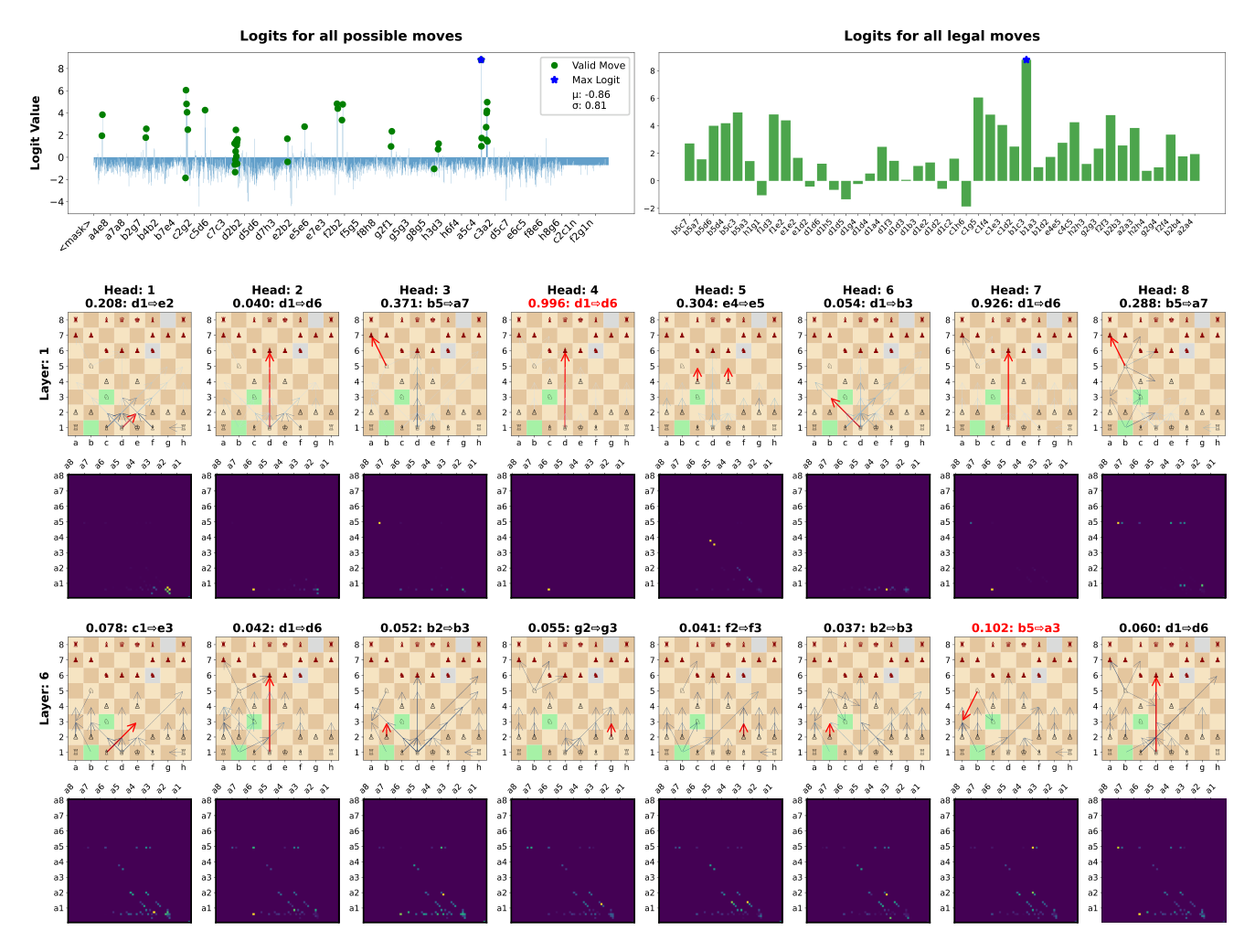
Several things are interesting in this image. First of all the logits are just showing high values for legal moves. As this model did not see this specific situation during training, the model learned statistical patterns consistent with legal move structure from the training data. Some legal moves have a negative logit value. This would not mean that the model would consider these moves illegal, but maybe just unpreferred in this situation.
The logit value of the played move shows a relatively high difference to the logit value of the next best move, suggesting the model’s high confidence in the chosen move. Furthermore, the selected move corresponds to the second-best move in the evaluation engine’s analysis for this position and the move played by the human player in this situation.
The attention values in the first attention layer are in certain attention heads considerably higher than in the last layer. Further, not many moves have a high attention in the first layer. In the last layer the attention is relatively higher on all moves in a head, visible by the darker color of the arrows on the board. This indicates that the attention becomes less focused on certain areas of the board, but more distributed over the whole board. This could indicate that the model first focuses on local patterns and then combines this information to a more global understanding of the board situation.
Lastly it is interesting that the attention of the played move is rather low in all heads of the last layer. This indicates that the feed forward network, which uses the attention as input, has a larger influence on the decision-making in this case.
Base UDRL architecture - baseline (2-4)
Now the first Upside Down Reinforcement Learning (UDRL) based models get evaluated. As mentioned, the encoder model was adjusted to a UDRL architecture, by adding the reward signal as input. The first experiment used the evaluation difference-based reward signal and the second one used the material difference-based reward signal. The third experiment then used the evaluation difference-based reward signal and added the information about legal moves during training.
2_UDRL-eval
The visualizations and results below show the results based on the UDRL architecture with the evaluation difference-based reward signal. For the visualization 100 matches per reward target have been played, this time just against Stockfish on level 3. The reward targets have been set ranging from -1 to +1 (inclusive), with a step size of 0,1. These reward target values were chosen according to the normalized reward signal which was used for training and was clamped between -1 and +1 (compare reward distribution). The resulting 21x100 games show how the playing strength of the model changes based on different reward targets and are visualized below.
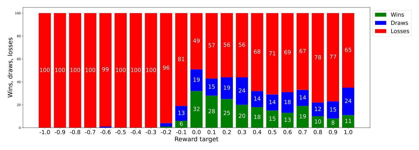
The plot demonstrates a clear influence of the reward signal on playing strength and that around a reward target of >= 0 the model started to win games against Stockfish. These results align well with how the reward distribution was built, with 0 being a move not affecting the evaluation and everything above 0 increasing the evaluation, therefore being a particularly good move.
The next table shows whether this model is able to play significantly differently than the Chess-Transformer architecture. This is compared for the reward targets -1, 0 and +1 for 500 games each. Both models played against Stockfish on level 3 as a shared benchmark, as they are not compared directly against each other, as mentioned.
| Reward signal | Model A | A: Wins / Losses / Draws | Model B | B: Wins / Losses / Draws | OR | p-value | Result |
|---|---|---|---|---|---|---|---|
| -1,0 | 2_UDRL-eval | 0 / 500 / 0 | 1_TEO | 115 / 303 / 82 | – | <0,001 | 1_TEO plays stronger. |
| 0,0 | 2_UDRL-eval | 143 / 244 / 113 | 1_TEO | 115 / 303 / 82 | 0,68 | 0,004 | 2_UDRL-eval plays stronger. |
| +1,0 | 2_UDRL-eval | 60 / 381 / 59 | 1_TEO | 115 / 303 / 82 | 2,09 | <0,001 | 1_TEO plays stronger. |
L3, 2_UDRL-eval with different reward targets compared to 1_TEO - source: own depiction
The next table checks if the model played significantly different for different reward targets. For this just the reward targets of -1, 0 and +1 are chosen and run for 500 games.
| Reward signal A | A: Wins / Losses / Draws | Reward signal B | B: Wins / Losses / Draws | OR | p-value | Result |
|---|---|---|---|---|---|---|
| -1,0 | 0 / 500 / 0 | 0,0 | 143 / 244 / 113 | 0,00 | <0,001 | Second plays stronger. |
| 0,0 | 143 / 244 / 113 | +1,0 | 60 / 381 / 59 | 3,06 | <0,001 | First plays stronger. |
L3, 2_UDRL-eval, with different reward targets - source: own depiction
Key findings:
With a set reward target of 0 the model is able to play significantly better compared to the base Chess-Transformer architecture. This answers the first research question, whether adding a reward signal can improve the playing strength of a Transformer-based chess model, positively.
For a negative reward target the 2_UDRL-eval model plays significantly worse than the 1_TEO model. For the reward target of +1, which should result in the strongest play, the 1_TEO model plays significantly stronger as well. This could be explained by the fact that a reward target of +1 is very rare in the training data (compare reward distribution) and therefore the model has problems adapting to this target. Further it may not always be possible to reach such a high reward in all states.
The differences in performance between the reward targets confirm that a reward signal can be used for steering the playing strength to a certain degree and therefore answers the second research question positively as well. However, the model seems to have problems reaching its full potential with very high reward targets, for the just mentioned reasons.
The following experiments analyze these findings further.
Reward target change during gameplay
Now the reward signal given to the model was changed during a single game to analyze how the model reacts to it. If the reward signal would have a direct influence on the playing strength during a game, this would show in different evaluations before and after the reward target change. Further that would confirm that the model selects individual moves based on the reward target.
In the first experiment the reward target was set to 0 for the first five moves and for the next five moves the reward target was set to -1. In the second experiment this was switched and the model started with the negative reward target. Both experiments have been run for 500 games. All games reached the 10 move mark. The distribution of the evaluation after the two phases is shown in the images below.
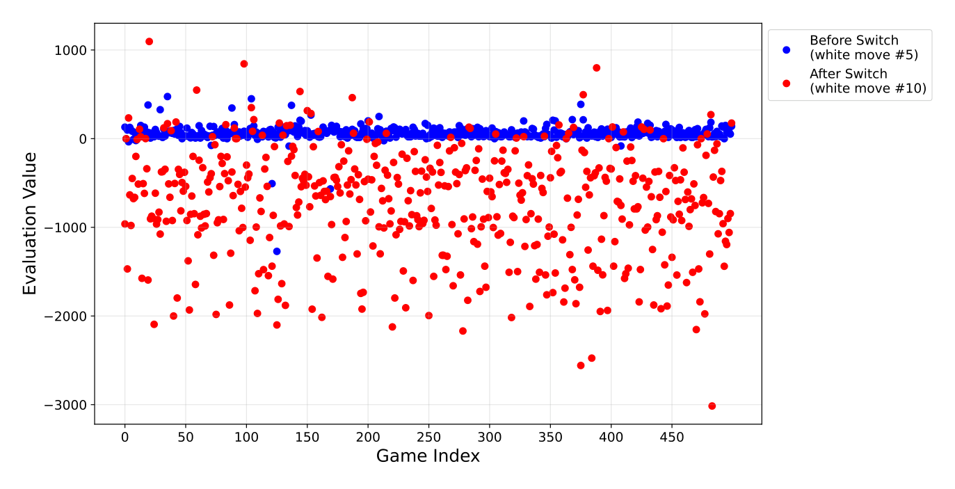
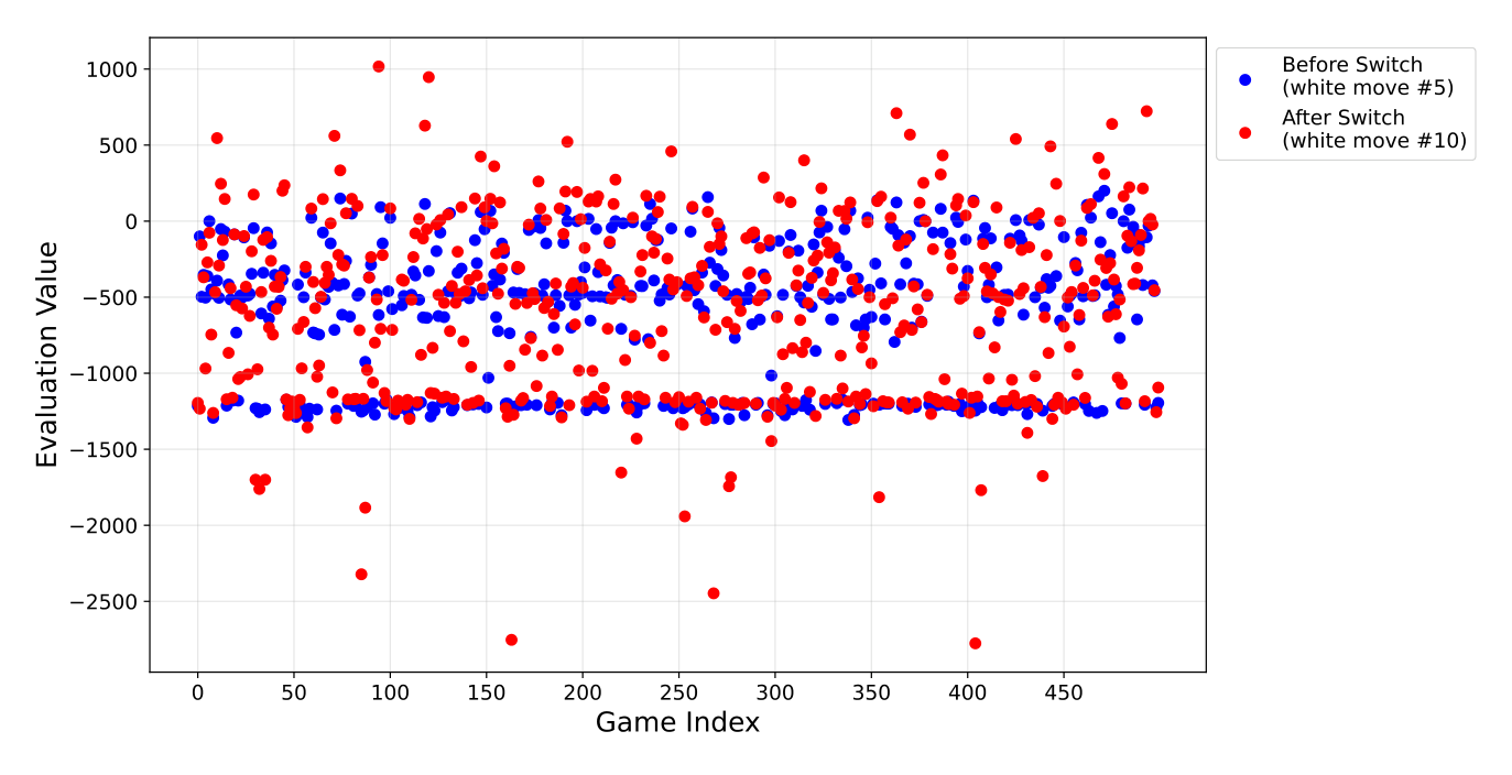
The first visualization shows the expected result, that the model plays better while a higher reward target is given and worse with a lower reward target. The second visualization shows no clear difference between the two phases, which is unexpected. This could be explained by the model having problems recovering from a bad position, as the difference in playing strength between this model with a reward target of 0 and Stockfish on level 3 is not large enough for the model to do so. The next table analyzes whether the shown differences are statistically significant via a Kolmogorov-Smirnov (KS) test.
| Sequence | Reward target | Mean | Std. | KS | p-value | Result |
|---|---|---|---|---|---|---|
| 0,0 to -1,0 | 0,0 | 66,35 | 97,38 | 1,00 | 0,00 | Null hypothesis of similar distributions is rejected. |
| -1,0 | -781,59 | 585,76 | ||||
| -1,0 to 0,0 | 0,0 | -640,41 | 454,83 | 0,40 | 0,31 | Null hypothesis of similar distributions can not be rejected. |
| -1,0 | -582,07 | 557,54 |
Evaluation change during gameplay with changing reward target for 2_UDRL-eval - source: own depiction
This test confirms the visualized results.
Key findings:
The significant change in average evaluation when switching the target from 0,0 to -1,0 confirms that the model is able to adjust its playing strength dynamically based on the reward targets, even within a single game, when starting with a higher reward target. This confirms the second research question and indicates that the model is indeed using the reward signal to take its decision for each move.
Analyze OOD reward targets
According to the literature the model should not be able to generate meaningful moves, if the reward targets are chosen outside of the training distribution. This would mean the model has never seen such a reward signal during training and can not infer an according move. As the reward targets have been normalized between -1 and +1 in the training data, everything outside of this range should be out-of-distribution (OOD). Therefore the model was tested with reward targets in the more negative and more positive range, with -1, 0 and +1 shown for comparison.
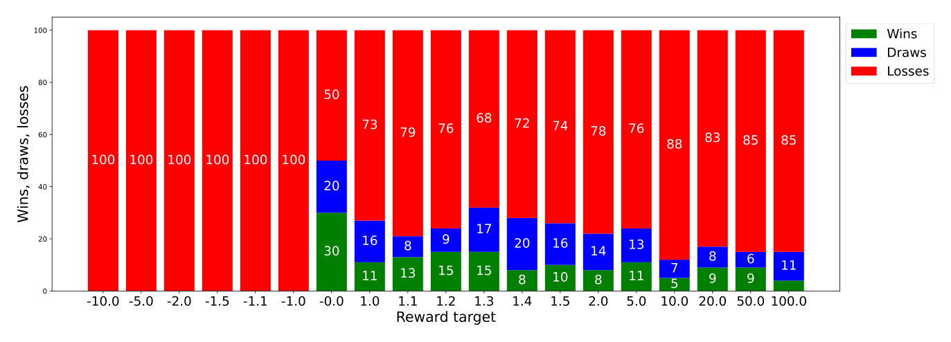
The results show that with negative OOD reward targets the model continues to play bad. For the positive OOD reward targets the model seems to continue to play comparable to the reward target of +1. The differences in playing strength was tested for statistical significance and is shown below.
| Reward signal A | A: Wins / Losses / Draws | Reward signal B | B: Wins / Losses / Draws | OR | p-value | Result |
|---|---|---|---|---|---|---|
| 1,0 | 60 / 381 / 59 | 1,5 | 51 / 381 / 68 | 1,06 | 0,739 | No significant difference. |
| 1,0 | 60 / 381 / 59 | 2,0 | 44 / 381 / 75 | 1,14 | 0,556 | No significant difference. |
| 1,0 | 60 / 381 / 59 | 5,0 | 53 / 392 / 55 | 1,14 | 0,500 | No significant difference. |
| 1,0 | 60 / 381 / 59 | 10,0 | 44 / 409 / 47 | 1,40 | 0,067 | No significant difference. |
L3, 2_UDRL-eval with different out-of-distribution reward targets - source: own depiction
So no difference between OOD values and the last in-distribution value of 1,0 could be found. With 10 as OOD value coming close to the p-value threshold. As the literature states that OOD reward targets should lead to poor performance and it was already assumed that +1 is a rare reward in the training data, it can be further assumed that +1 is already somewhat of an OOD target. Therefore another experiment testing the OOD criteria was conducted later (compare 8_UDRL-eval-manipulated_reward).
Key findings:
The results show that for positive OOD reward targets do not significantly worsen the play compared to the last in distribution reward target. A possible explanation could be that a reward target of +1 is already playing significantly worse then the reward target of 0. Looking at the initial reward distributions, which shows that +1 is a very rare reward in the training data, it could be argued that the +1 is somewhat of an OOD target already.
Analyze attention weights
Next the attention weights of the model were analyzed. The image below shows a full visualization of the discussed move and the associated attention and logits by the model, with a reward target of 0.
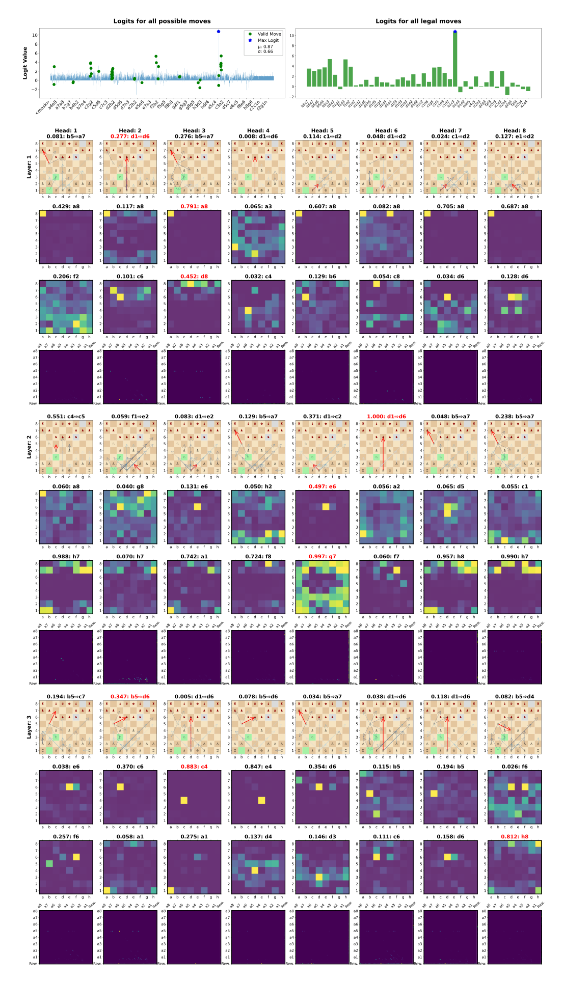
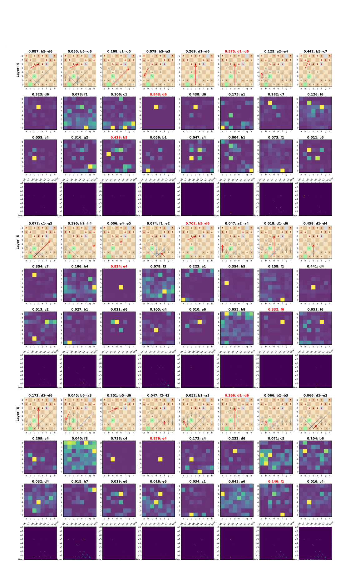
In this image the logits look quite different from the previous model. Here almost all logits are positive, with the logit values for legal moves being somewhat comparable in difference and the selected best move having an even higher difference to other legal moves, indicating that the model is even more sure about this move.
In layer 1 the attention is with regards to its distribution comparable to the 1_TEO model. Especially noticeable is that the attention pattern in the heads 2 and 3 in the 1_TEO model are very similar to the heads 4 and 2 in this model. This could indicate that these heads learned similar patterns in both models.
Across layers mostly one or two heads have a distinctively high attention, compared to the other heads in the layer, with the specific head with the highest attention switching between layers. This would indicate the model not being very sure about the attention.
In layer 5, head 5 and 8 the reward query shown in the visualization appears to focus on high value pieces to take. This aligns very well with the square attention in the same layer and heads. In the last layer the highest reward key attention focuses on the source square of the executed move. This does not align with the square attention, but is the move that was picked by the model.
The next two images show the attention and logits for the same move, but with reward targets of -1,0 and +1,0.
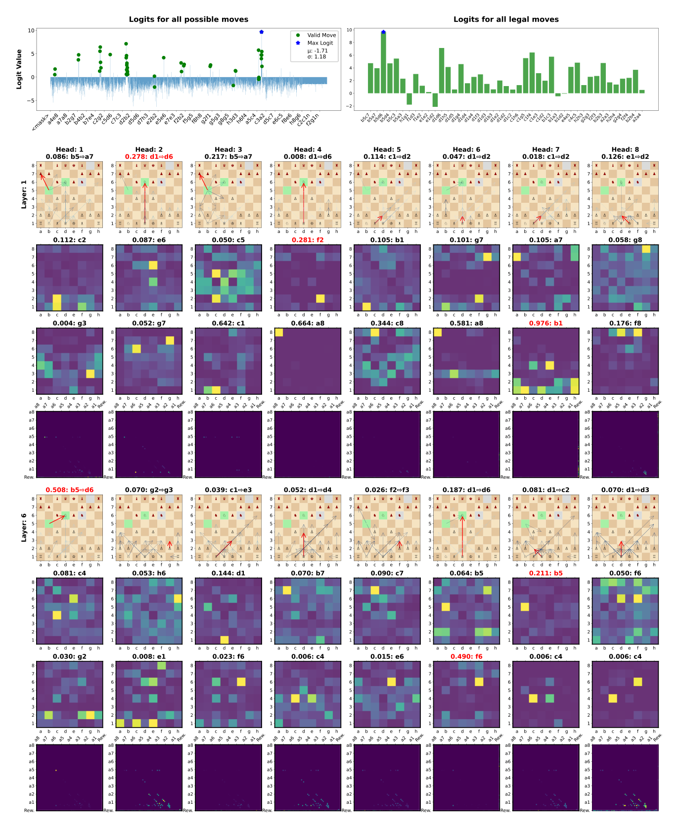
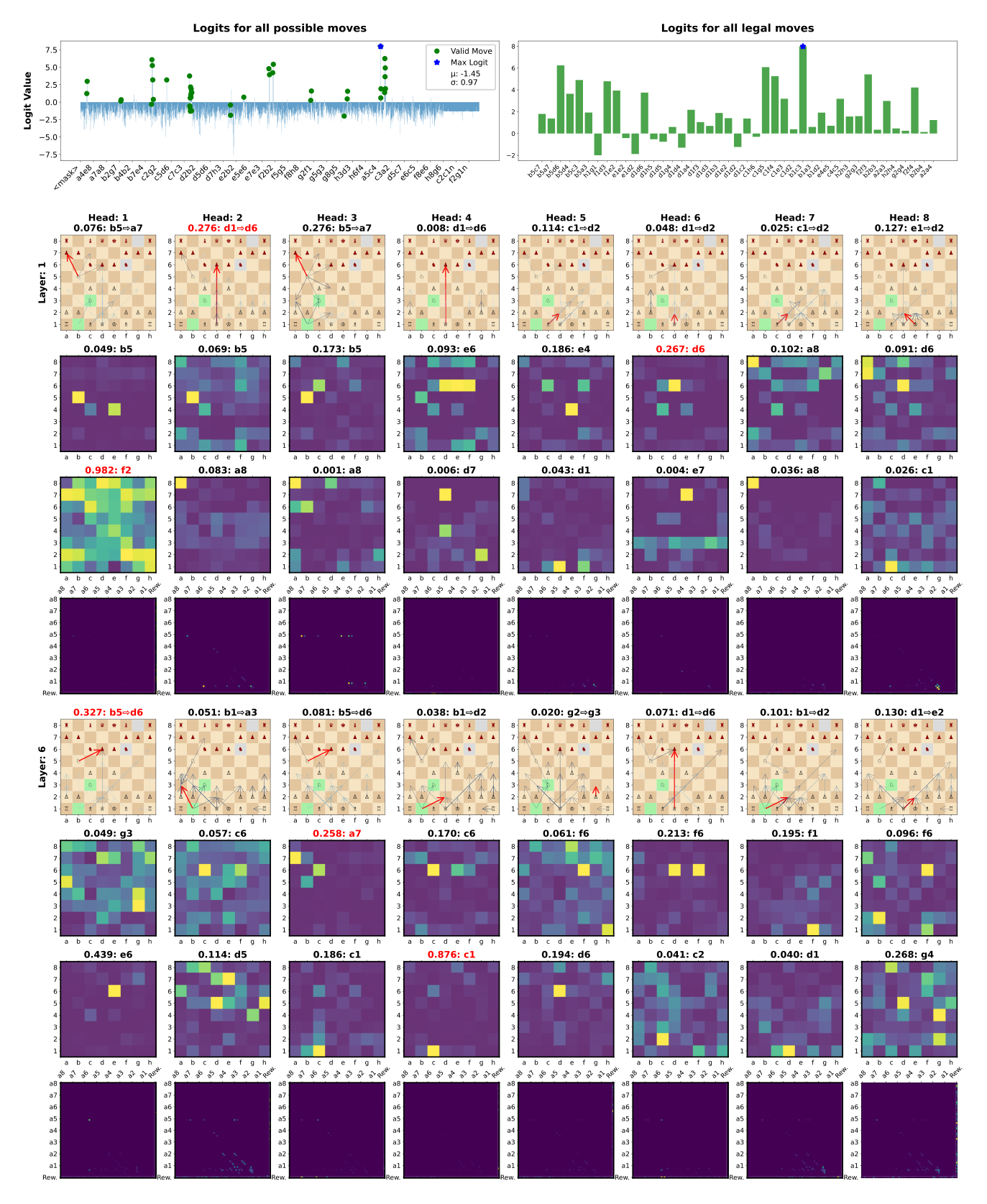
Here the logits show a similar pattern than in the first model. With almost all illegal moves having a negative logit value. In distinction to the earlier shown reward target of 0, which has the highest playing strength, could indicate that higher overall logits are not an advantage. Further the position played with a reward target of -1 did decide on a non-optimal move, which is also reflected in the logits. Here the difference in the logits is not as high as in the game with a reward target of 0. For the reward target of +1 the logits for legal moves are closer together as well. This shows that the model is less sure about the move selection in this case. The other parts of the image are not very different to the earlier shown reward target of 0.
In these visualizations, where the set reward target is at the fringe of the reward distribution, the reward attention is not that clearly focused as before. No clear pattern can be derived from these images. With the reward attention for the reward target of -1 all over the place.
In experiment 4_UDRL-eval-legal_input these visualizations are analyzed without a mask on illegal moves and shown for this model in comparison. Then further assumptions about the function of the attention can be derived.
3_UDRL-material
Here the UDRL model with a material difference-based reward signal was analyzed. The following visualization shows again the model’s results against Stockfish on level 3, with target rewards between -1 and +1, in steps of size 0,1, for 100 games each.
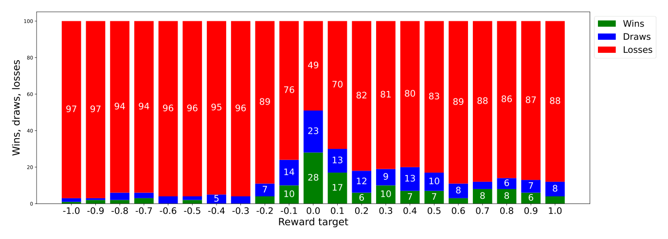
Here the playing strength of the model seems to be roughly comparable to the evaluation-based UDRL model, at least for the reward target 0. The ability to steer the model is visible as well, with a stronger play closely around a reward target of 0 and falling off faster for the more positive targets. The results were tested for statistical significance against the evaluation difference-based UDRL model and are shown in the tables below for selected reward targets.
| Reward signal | Model A | A: Wins / Losses / Draws | Model B | B: Wins / Losses / Draws | OR | p-value | Result |
|---|---|---|---|---|---|---|---|
| -1,0 | 3_UDRL-material | 0 / 500 / 0 | 2_UDRL-eval | 0 / 500 / 0 | – | 1,000 | No significant difference. |
| 0,0 | 3_UDRL-material | 155 / 236 / 109 | 2_UDRL-eval | 143 / 244 / 113 | 1,09 | 0,562 | No significant difference. |
| +1,0 | 3_UDRL-material | 22 / 443 / 35 | 2_UDRL-eval | 60 / 381 / 59 | 0,39 | <0,001 | 2_UDRL-eval plays stronger. |
L3, 3_UDRL-material compared to 2_UDRL-eval, with different reward targets - source: own depiction
The results show that the material difference-based reward signal performs very similarly to the evaluation difference-based reward signal for the reward target 0. It performs slightly stronger for lower reward targets and slightly weaker for higher reward targets. This aligns well with the expectation, as the material difference-based reward signal shows a stronger peak at 0 and less extreme values of +1 and -1, making them rarer in the training data, compared to the evaluation difference-based reward signal.
Next the inference plots for the reward targets -1,0, 0,0 and +1,0 are shown for the same move as before, again with masked attention for legal moves.
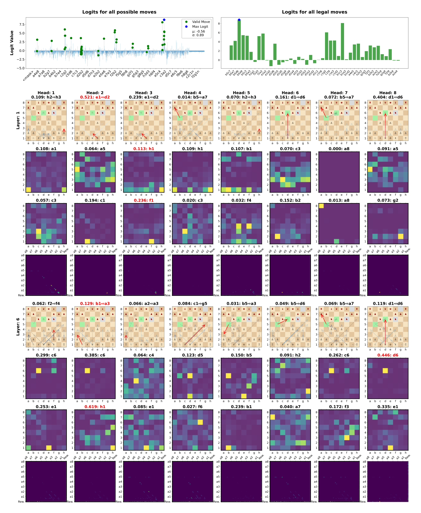
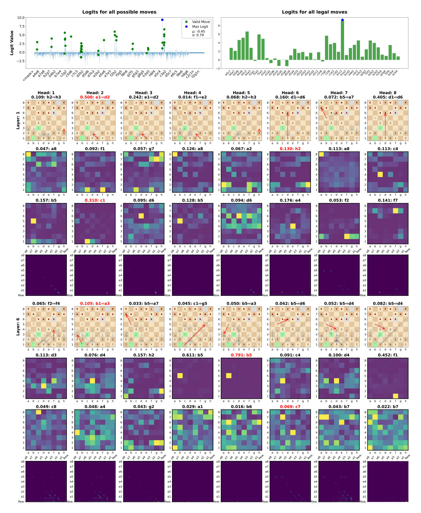
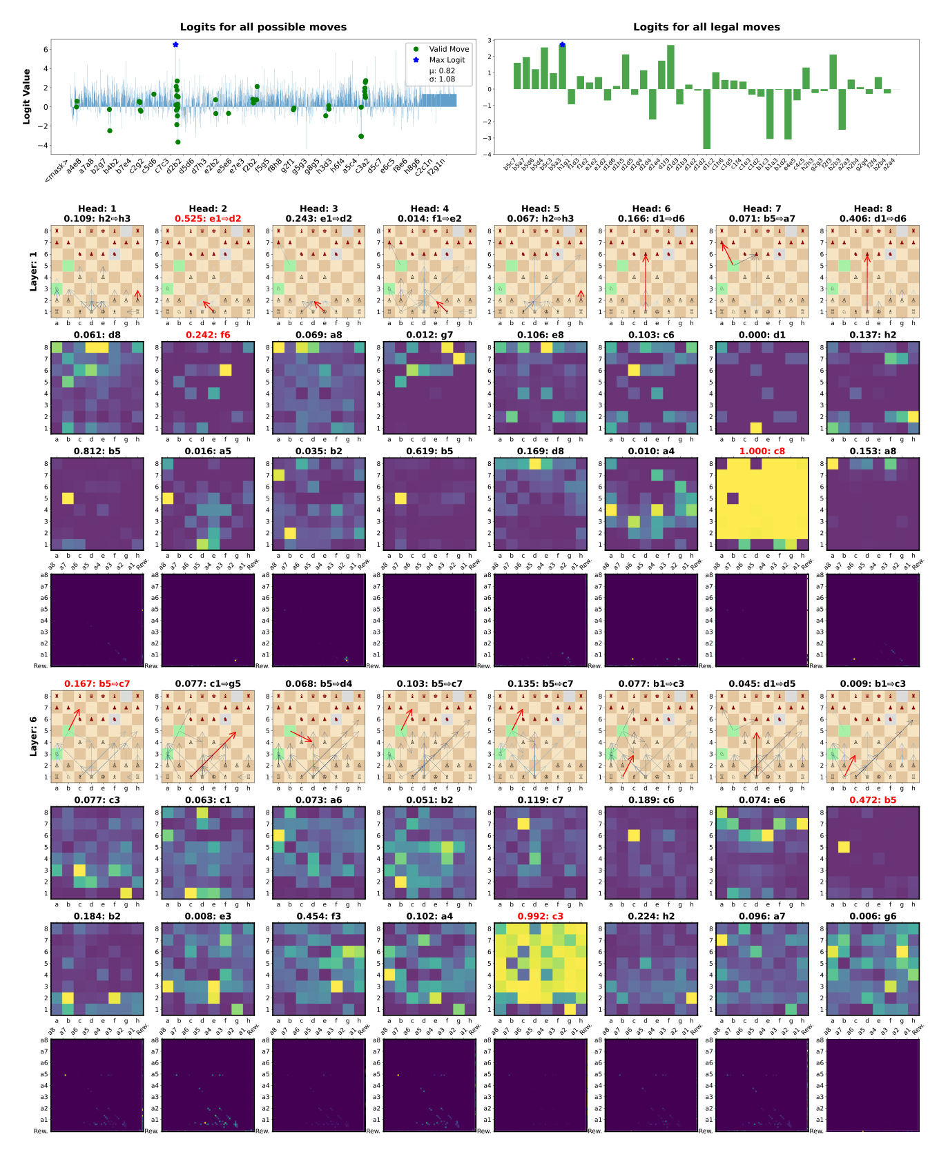
Here the logits show a similar pattern as in the evaluation difference-based UDRL model. The game played with a negative reward target shows the logits of all legal moves closely together. The game played with reward target 0 does not show the distinctive positive logits for most moves as the earlier model did. Further the logit for the game played with reward target +1 do not show a clear distinction between legal and illegal moves anymore. This could indicate the model not having this reward target as part of its learned distribution.
For the reward target -1 the model picks the move with the highest reward query attention on the target square of the move (d6). That is not the case for the reward target of 0, where the reward query attention focuses on a different square and the reward key attention shows no clear picture, again indicating that the following feed forward network has a stronger influence on the decision making. The reward attention for the reward target -1 is again all over the place.
Key findings:
The material difference-based reward signal shows a similar effect than the evaluation difference-based signal, by showing the ability to adjust the playing strength based on the target reward. Further it was able to play on a similar level than the 2_UDRL-eval model for a reward target of 0, but not for a reward target of +1. A possible reason for this could be that the reward signal is more closely spread around 0 with a standard deviation of 0,129 for the material difference-based signal, compared to 0,244 for the evaluation difference-based signal (compare reward distribution). This would make it harder for the model to adapt to higher reward targets, as these were seen less.
4_UDRL-eval-legal_input
Based on the findings of the first experiments this experiment was designed to provide additional information about how the architecture makes decisions. Until now the models did not have information about which moves are legal in a given board state during training, but were just given a single action in the specific situation as input, which was then optimized against. There are multiple possibilities to provide the other legal moves to the model. One method would be masking illegal moves via setting their attention weights to zero before the feed forward network uses the attention. Another method, which was implemented here, is adding the legal moves as an additional feature vector, which is then embedded and used as further input dimension alongside the state and reward. This requires the legal moves to be calculated and provided during both training and inference, which has been adjusted accordingly in the model and data pipeline.
This experiment should provide more information about the steering capabilities, as the model should be able to focus on legal moves more easily with this additional information. If this experiment succeeds, other steering scenarios could be possible as well, e.g. focusing on moves of a specific piece type.
The results of this experiment are visualized below, again via playing 100 matches against Stockfish on level 3 with target rewards between -1 and +1, in steps of size 0,1 and adding the legal moves as input for each move.
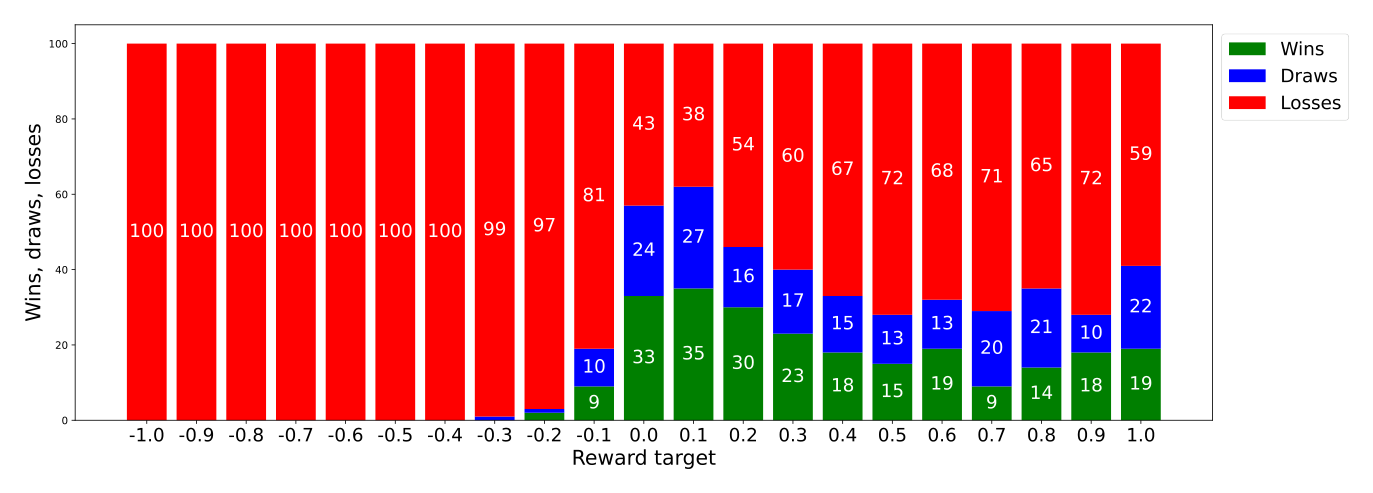
The visualization indicates an improvement in playing strength for reward targets of 0 and above, compared to the earlier models. As always statistical tests were conducted to verify this.
| Reward signal | Model A | A: Wins / Losses / Draws | Model B | B: Wins / Losses / Draws | OR | p-value | Result |
|---|---|---|---|---|---|---|---|
| -1,0 | 4_UDRL-eval-legal_input | 0 / 500 / 0 | 2_UDRL-eval | 0 / 500 / 0 | – | 1,000 | No significant difference. |
| 0,0 | 4_UDRL-eval-legal_input | 163 / 208 / 129 | 2_UDRL-eval | 143 / 244 / 113 | 1,26 | 0,084 | No significant difference. |
| 1,0 | 4_UDRL-eval-legal_input | 77 / 339 / 84 | 2_UDRL-eval | 60 / 381 / 59 | 1,44 | 0,024 | 4_UDRL-eval-legal_input plays stronger. |
L3, 4_UDRL-eval-legal_input compared to 2_UDRL-eval, with different reward targets - source: own depiction
While the visualization let a stronger play appear to be the case and the test for the reward target of 0 came close to confirm this, adding the information about legal moves to the model has no statistical significant impact on the playing strength for the reward target 0. For the reward target of +1 a significant improvement could be found, indicating that the model is better able to adapt to this rare reward target with the additional information.
Below the inferences for these models are shown. These plots are not masked to just show legal moves but instead show all moves the model considered. For comparison the non-masked inferences for 2_UDRL-eval are shown.
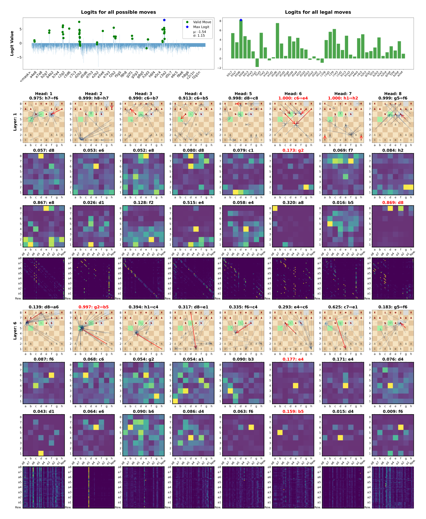
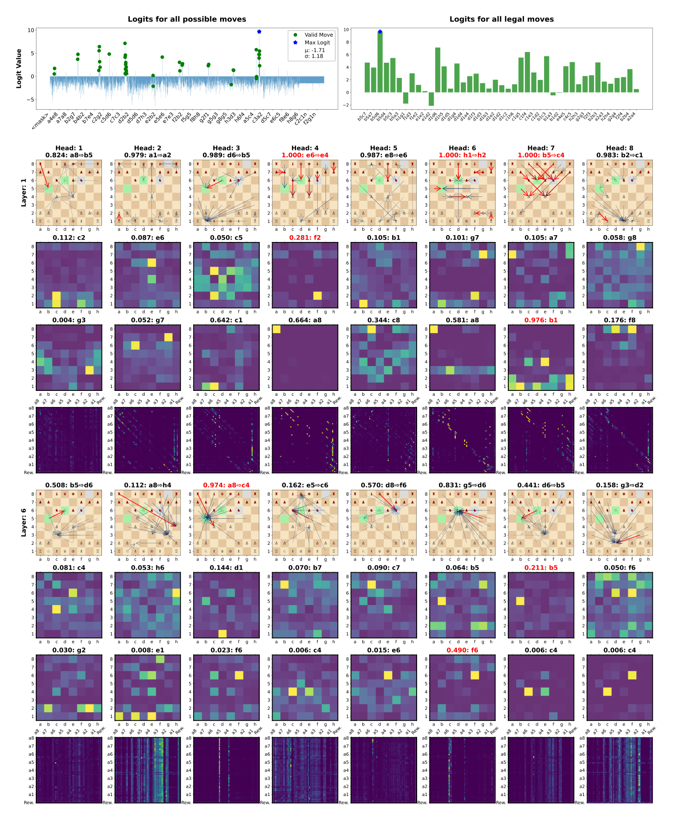
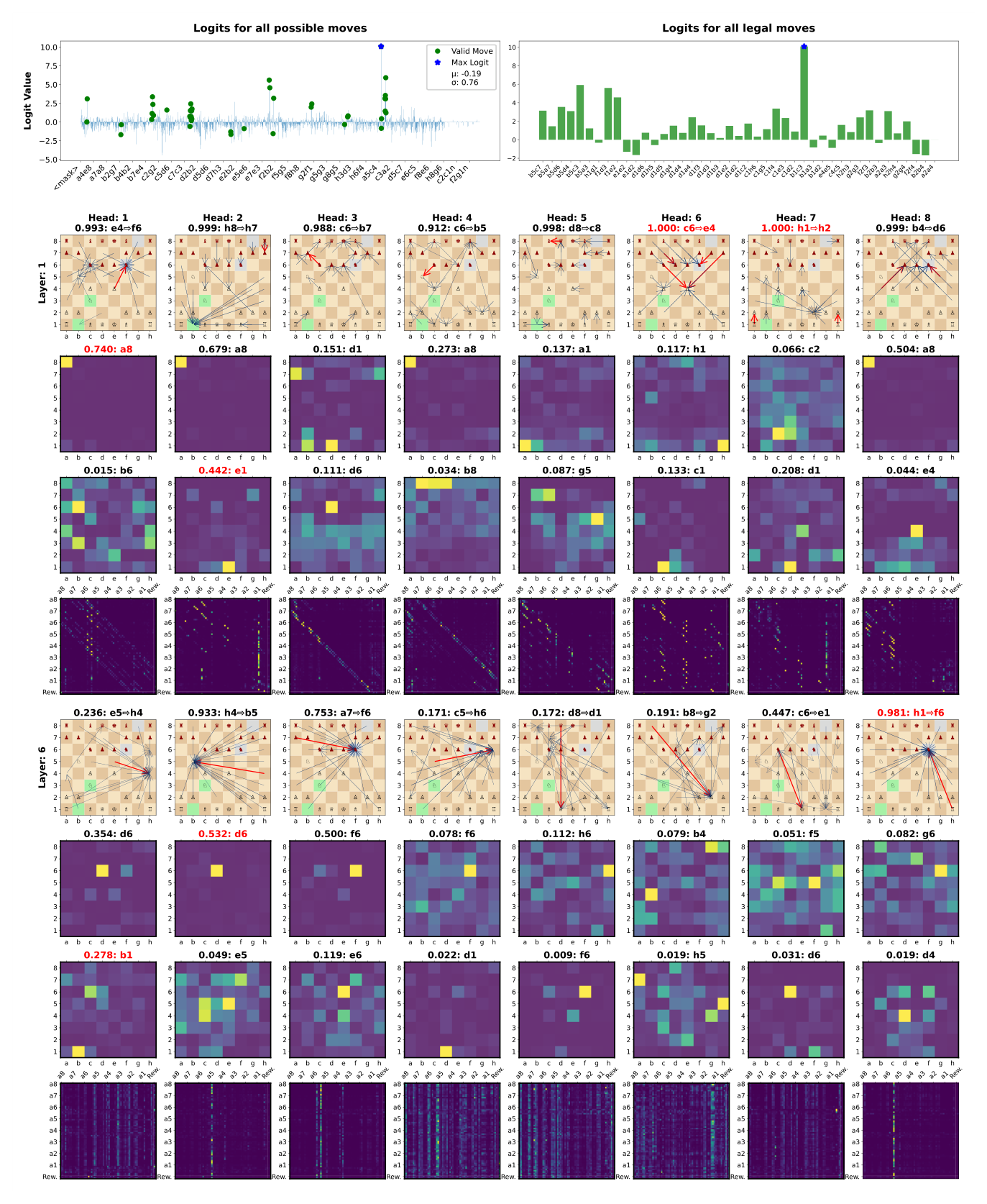
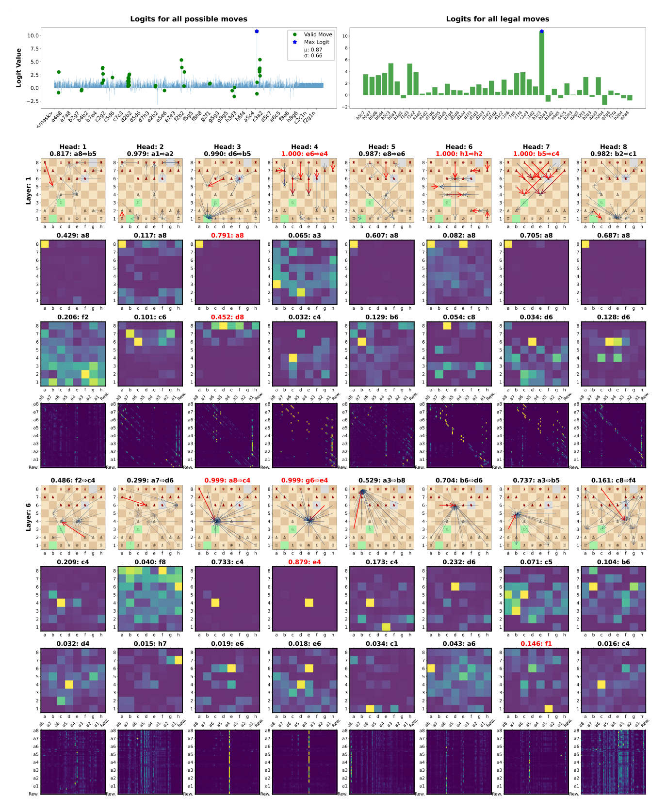
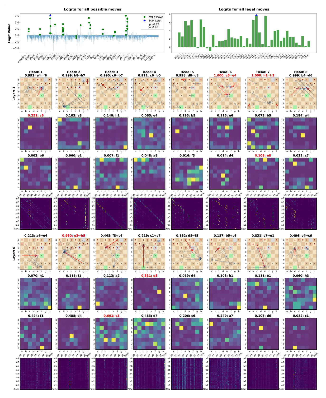
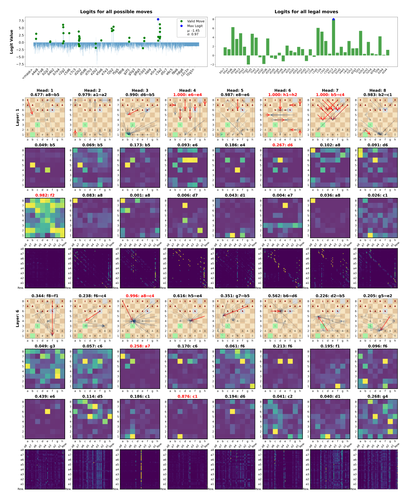
For this model the attention values shown on the board do not seem to focus much on legal moves but are all over the place. There seems to be no distinction to the 2_UDRL-eval model, which did not have the legal moves as input. This suggests the 4_UDRL-eval-legal_input model does not rely much on the legal move information in the attention. Both models show similar attention patterns in the first and last layer, with the first layer focussing on diagonal relationships between squares and the last layer focussing on the source square of the played move. Further the non-masked inferences show that the attention is overall not sparse, but distributed over many squares.
The reward attention for the reward target of -1 and 0 again focuses on the source square of the played move in the last layer, while the model picks a different move for each reward target. The reward attention for the reward target of +1 shows no clear pattern again.
The following plots show the legal move input embedding mapped to the board squares, comparable to the reward key and query inferences.
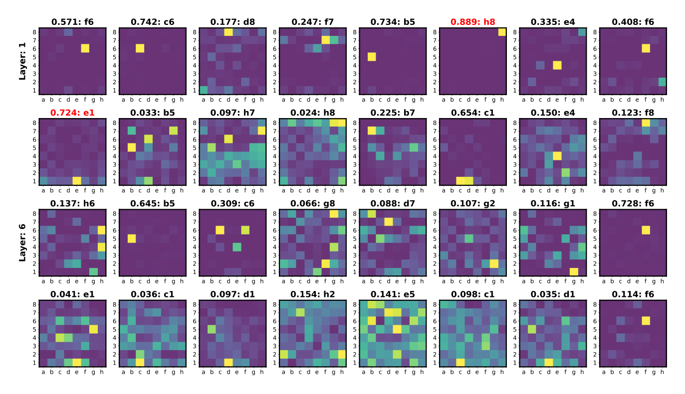
For the legal information the first layer shows again a rather localized pattern, while the last layer shows a more distributed pattern. Overall no clear conclusion can be drawn from these images.
Key findings:
Adding the explicit legal move information did not succeed in localizing the attention weights exclusively to legal moves. It did not improve playing strength significantly either, but still showed some improvement. A possible explanation for this could be that the model already learned to focus on legal moves quite well without this additional information, as illegal moves are not rewarded during training. Therefore adding this information does not provide a significant advantage.
Continue with Part 4: Results - reward targets, manipulation and conclusion, which covers the Return-To-Go models, the Decision Transformer, the reward manipulation experiments, the Elo signal model, the discussion and the conclusion.
References
The training was executed on rented cloud instances, which did not always provide a consistent environment, besides the GPU specification. As some data processing was executed during training, the data loading was rather CPU intensive. ↩︎
The project provides the training logs as Tensorboard files for download: https://github.com/sgrvinod/chess-transformers?tab=readme-ov-file#ct-e-20 ↩︎