Transformer-based ORL Applied to Chess - Part 2: Experimental Setup
Master Thesis, Part 2: Eleven models, the evaluation against Stockfish, the codebase and the reward distributions
Table of Contents
This section introduces the experiments designed to analyze the defined research questions. First, the different experimental setups are introduced, followed by the evaluation methods. Afterwards, the codebase and the training data will be discussed, together with the distribution of the two reward types used throughout the experiments.
About this paper
Master Thesis for the Master of Science - Artificial Intelligence at IU International University.
The original LaTeX source, the bibliography, the full code, the data preparation and the compiled PDF are available on GitLab: gitlab.com/iu-msc-ai/transformer-based-offline-reinforcement-learning-applied-to-chess
This is part 2 of 4:
- Foundations
- Experimental setup (this part)
- Results - Chess-Transformer baseline and base UDRL
- Results - reward targets, manipulation and conclusion
Experiments and evaluation
In this section, the experiments are presented. Several models have been designed and trained, each with the goal of investigating a different part of the research question. The experimental setup has multiple dimensions and is discussed in the following. An overview of the different experimental dimensions is shown below.
- Model architecture: Transformer (encoder-only) from Chess-Transformer, Upside Down Reinforcement Learning (UDRL) and Decision Transformer (DT) architecture
- Reward type: evaluation difference-based or material difference-based reward
- Reward trajectory: single-step reward vs. cumulative reward over a longer trajectory (return-to-go, RTG)
- Trajectory length: different trajectory lengths for the RTG
- Legal move information: adding the legal moves as input to the model
- Elo signal: changing the move based rewards to the Elo of the player making the move
- Special setting: blocking a specific move via manipulating the reward or removing the action from the training data
1) Model architecture. The model architecture mainly differs in whether and how the rewards, states and actions are incorporated into the model. Three different architectures were tested here. A baseline architecture without any reward signal, similar to a standard supervised learning (SL) setup, where just the current state is used to predict the next action. This architecture is based on the original Transformer architecture implemented in the Chess-Transformer project. Then the UDRL architecture, where a reward signal is added as input to the model, to be able to condition the action prediction on a desired reward. Further, a DT architecture was tested, where reward, state and action trajectories are used to predict the next action.
2) Reward type. The reward type defines how the reward is calculated during training and inference. There are multiple possibilities to do this. Here always one of two following types is used. The difference between these two reward types was then analyzed in regards to their impact on the learning process and playing strength.
One classical way to evaluate a board state is by material difference. Each piece has a certain value assigned to it. Commonly a pawn gets a value of 1, a knight a 3, a bishop a 3, a rook a 5 and a queen a 9. The king does not have an assigned value, as the game automatically ends when the king is captured. By calculating the difference in material balance before and after a move, a reward can be assigned. This is a rather simple and computationally cheap way to evaluate a chess position. It does not take into account positional advantages or disadvantages though.
However, for evaluating a white move, simply using the material difference after the move is insufficient, as this would lead to just positive rewards for any move, as it ignores a possible capture by black. To mitigate this, the difference in material balance across both players’ moves was used as the reward signal. Therefore, this reward mixes white and black moves and would add a possible very good or bad black move into the reward signal.
The other implemented reward type is a reward based on a chess engine’s evaluation. In this case a highly capable chess engine, like Stockfish, evaluates a board position by playing out the current situation for a limited amount of steps, called depth, in a predefined amount of time. The chess engine acts as a strong external evaluator, which is comparable to a complex reward function used in other reinforcement learning (RL) problems. The evaluation is usually given in centipawns, which is based on the just mentioned material difference logic. A pawn, valued at 1, gets the value 100, so one point is a hundredth of a pawn. A positive evaluation means that white is better, while a negative evaluation means that black is better. An evaluation of 0 means that the position is equal. If the engine detects a possible mate it does not provide a centipawn evaluation anymore, but just the number of moves left. In this case, the evaluation value was set to ± 250 centipawns, as this was deemed a realistic value found in the dataset for comparable high superiority positions. Then a difference is calculated between the evaluation value before and after the move. A positive difference means that the position improved for the player making the move, while a negative difference means that the position worsened. In chess it is in general harder to improve a position than to worsen it. The resulting distribution of this reward signal is analyzed later (compare reward distribution).
Another way of building a reward signal would be to use the game result as reward. This would be a very sparse reward signal though, as only the final move of the game would provide a non-zero reward, which then would be backpropagated to all previous moves. This would make the learning process very difficult, as the model would struggle to identify which high impact actions led to the final result. Early experiments with such a reward structure did not show promising results. Therefore this approach is not used here. Instead, the RTG provided a middle ground between the sparse game-result reward and the immediate per-move reward signal. This will be discussed next.
3) Reward trajectory. The reward was calculated either for a single-step reward trajectory, focusing only on the current move’s immediate reward or for a longer reward trajectory using the RTG approach. The RTG was calculated as the undiscounted sum of the current move reward and future rewards, similar to the approach mentioned in the DT architecture. Different trajectory lengths were tested as well, to analyze their impact on the learning process. Models using these different trajectory lengths were then compared against each other.
4) Legal move information. Adding information about legal moves for the specific state was tested by using the legal moves available in the individual state as additional input. This provides another signal to the model, which can help to improve the learning process and playing strength. It was tested if the model benefits from this explicit input during training and inference and if the attention mechanism would reflect this information.
5) Elo signal. The Elo signal was tested as a replacement for the reward signal. The Elo signal could be considered a different measure of the playing strength of the player and therefore should correlate with the move quality of a player. Without a reward signal, the model is considered a standard SL setup again. The focus was on analyzing if the Elo signal has an impact on the learning process, in a similar fashion as a reward signal.
6) Special setting. Two special configurations were tested, one where the reward for specific moves was manipulated during training and a second where specific actions were removed from the training data. This was used to test whether the models effectively incorporate the reward signal into their decision-making.
The following table shows the individual models, their reward configurations and the name under which they are referenced later and under which name they can be found in the code repository. Not all possible combinations of the introduced dimensions have been included here, to keep the amount of models manageable and focus on the most interesting setups.
| Nr. | Model name | Model type | Reward signal | Comment |
|---|---|---|---|---|
| 1 | 1_TEO | Transformer (encoder-only) | – | This architecture is based on the Chess-Transformer project. |
| 2 | 2_UDRL-eval | UDRL | evaluation difference-based | |
| 3 | 3_UDRL-material | UDRL | material difference-based | |
| 4 | 4_UDRL-eval-legal_input | UDRL | evaluation difference-based | This architecture adds legal move information as input. |
| 5 | 5_UDRL-rtg3_eval | UDRL | evaluation difference-based RTG, 3 moves | |
| 5b | 5b_UDRL-rtg5_eval | UDRL | evaluation difference-based RTG, 5 moves | |
| 6 | 6_UDRL-rtg3_material | UDRL | material difference-based RTG, 3 moves | |
| 6b | 6b_UDRL-rtg5_material | UDRL | material difference-based RTG, 5 moves | |
| 7 | 7_DT-eval | DT | evaluation difference-based RTG, 3 moves | This architecture adds a state-action-reward trajectory as input. |
| 8 | 8_UDRL-eval-manipulated_reward | UDRL | evaluation difference-based | This architecture manipulates the reward for specific actions. |
| 9 | 9_UDRL-eval-hidden_action | UDRL | evaluation difference-based | This architecture removes specific actions from the training data. |
| 10 | 10_TEO-Elo_signal | Transformer (encoder-only) | – | This architecture adds the players Elo as input. |
Overview of trained models - source: own depiction
Each of these models are available as configuration files, which can be used to start or continue training of the respective model.1 The trained models were uploaded to a “Hugging Face” repository.2 Below the hyperparameters used for training the models are shown.3
| Hyperparameter | Value |
|---|---|
| Learning rate | 0,001 (0,0003 for DT) |
| Learning rate scheduler | Vaswani (linear decay for DT) |
| Warmup steps | 8.000 |
| Batch size | 512 |
| Batch accumulation | 4 |
| Number of layers | 6 |
| Number of heads | 8 |
| Embedding dimension | 512 |
| Fully connected dimension | 2.048 |
| Dropout rate | 0,1 |
| Optimizer | AdamW |
| Criterion | Cross-Entropy Loss |
| Dataset size | 500.000 games with >16 million moves |
| Training samples | 9 million moves |
| Evaluation samples | 1 million moves |
Hyperparameters for trained models - source: own depiction
These hyperparameters fall within comparable ranges to similar projects mentioned earlier (compare Transformer architecture). The batch size of 512 and the batch accumulation of 4 did result in an effective batch size of 2048 samples per weight update. Together with the 9 Million training samples this resulted in 4.394 weight updates per epoch.
Playing strength evaluation
For each architecture and tested configuration the playing strength was evaluated. The models played against the Stockfish chess engine on a selected playing strength setting. For models incorporating a reward signal, testing was conducted across multiple target rewards to analyze how the model adapts its play to these external commands. The results were visualized using bar charts for each experiment, with each setting played 100 times for a preliminary analysis.
Further, the results were compared against each other and tested for statistical significance, to determine if a difference in playing strength is significant or due to chance. This was performed by using a Fisher’s Exact Test, as the results are categorical, with wins, draws and losses. The draws were split evenly between wins and losses for the statistical test, as draws provide a half point to each player in chess. This provides binary results (win/loss), which can then be tested via Fisher’s Exact Test. As some categories had low frequencies a Chi-Square test was not deemed appropriate.4
The null hypothesis is that there is no difference in playing strength between the two tested models, while the alternative hypothesis is that there is a significant difference in playing strength. The applied test is two-tailed, allowing for the identification of which model is significantly stronger, if a difference exists. A significance level of $\alpha = 0,05$ was used for the tests.
As test statistic the Fisher’s Exact Tests odds ratio (OR) was used, shown below.5
$$ OR = \frac{\text{Group A (wins)} \times \text{Group B (losses)}}{\text{Group B (wins)} \times \text{Group A (losses)}} $$
Here Python’s Scipy libraries implementation of the Fisher’s Exact Test was used.6 The test takes as input a 2x2 contingency table, which summarizes the results of the two models being compared. The table contains the number of wins and losses for each model. The test then calculates the p-value, which indicates the probability of observing the given results under the null hypothesis.
from scipy.stats import fisher_exact
contingency_table = [
    [wins_A + (draws_A * 0.5), losses_A + (draws_A * 0.5)],
    [wins_B + (draws_B * 0.5), losses_B + (draws_B * 0.5)]
]
odds_ratio, p_value_fisher = fisher_exact(contingency_table, alternative='two-sided')
Fisher’s Exact Test implementation in Python - source: own depiction
For each comparison the models played 500 times against Stockfish, to increase the statistical power of the test. This comparison was just made for selected reward targets, which were deemed relevant from the visualizations.7 Mostly the reward targets of -1, 0 and +1 were tested. Therefore the models were not played directly against each other, but instead got compared based on their performance against Stockfish, acting as the benchmark.8 This makes comparisons between different configurations implicitly comparable.
The Stockfish engine can play and evaluate chess games on different levels of strength. The levels limit the full capability of the engine via limiting its search depth and calculation time per move. The skill levels can be mapped to approximate Elo ratings according to the following graphic provided by the Stockfish project.9
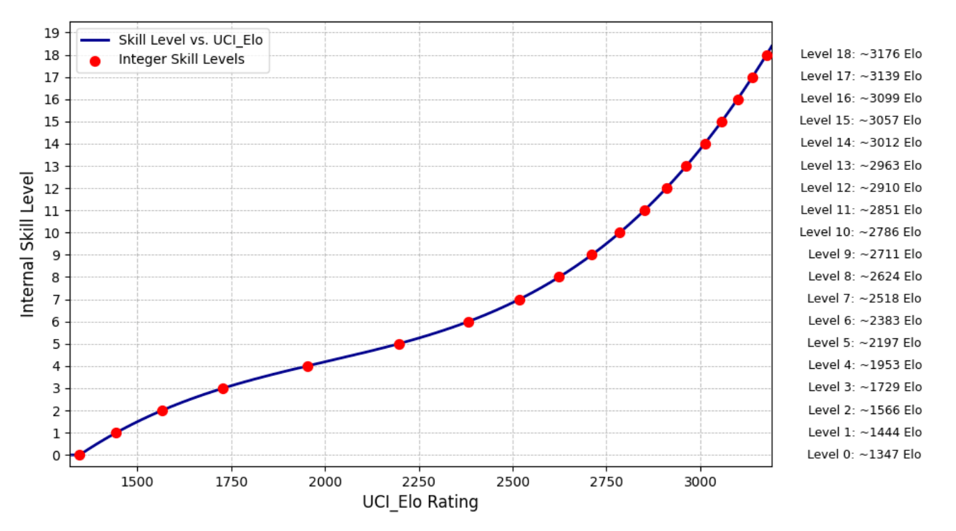
Here the Fairy-Stockfish engine, which is derived from Stockfish, was used, in its version 14.0.1.10 Level 3 was selected as the primary benchmark for most models. To calibrate this choice and validate level 3 as an appropriate performance baseline, the 1_TEO model was evaluated against levels 2, 3, and 4, which map to an Elo of approximately 1566, 1729 and 1953 respectively.
Attention and logit visualization
This section provides a general overview of how attention and logits are visualized, to infer insights into the model’s decision-making process during inference. Illustrative examples are provided here, while the experimental visualizations are presented in the result sections later. Visualizing the attention weights can provide insights into how the model focuses on different inputs during decision-making and could show correlational patterns, but should not be interpreted as causal explanations. A main part in the attention visualization is the source and target squares of the board, which are reflected by the queries and keys in the attention mechanism. Further the reward token is analyzed in detail, to see how the model incorporates the reward signal into its decision-making. In this case the reward token acts as either a query for the keys of the board squares or as a key for the queries of the board squares.
Analyzing the attention patterns across the different layers of the model can show how the attention changes from local interactions between pieces in early layers and more global patterns in later layers. The different heads of the model are able to focus on different things altogether. For example a single head might specialize on focusing on straight-line movements (e.g. for a rook) and another on diagonal movements (e.g. for a bishop or a queen), which would show a distinctive pattern in the attention matrix.
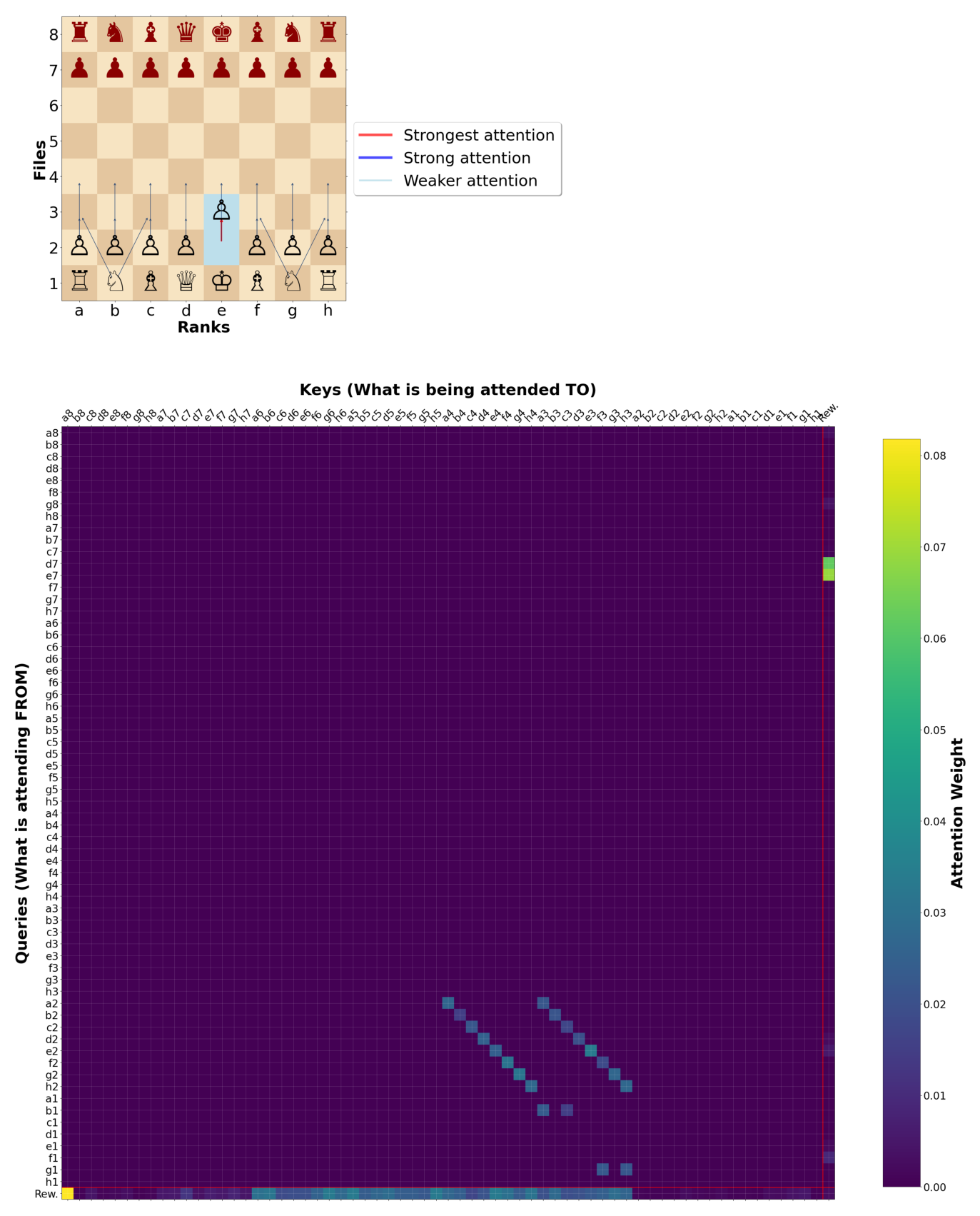
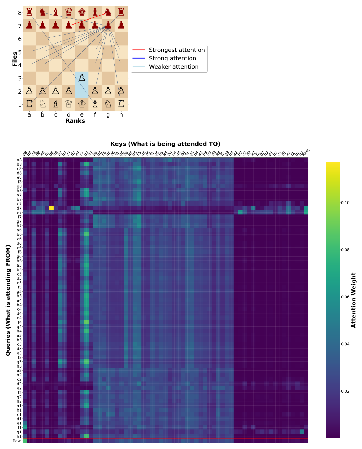
The attention visualizations reflect the raw multi-head attention scores, computed by taking the dot product of the query and key vectors, followed by a softmax operation to normalize the weights (compare attention mechanism). On these attention values a filter can be applied to display only the attention weights corresponding to legal moves. This would be done by setting the attention weights of illegal moves to zero just for the visualization and therefore apply a mask on illegal moves. This can be configured in the evaluation code for each visualization independently and was done to provide a clearer picture for the reader.11 The images below show a masked and not masked attention matrix.
One way to visualize the attention is as a matrix, where the rows represent the queries and the columns represent the keys. The attention matrix is then visualized as a heatmap, where the color intensity represents the attention weight. The classical “viridis” color map is used as the color scheme. To avoid overly extending the visualizations, the “viridis” color bar is shown only in the two examples below.
In chess it is simple, in distinction to other game environments, to show the attention on the game’s environment, which is the chess board. For each model the embeddings of the board squares kept the same dimensionality as the input of the 64 (8x8) board squares. Therefore, the dimensionality of the queries and keys are the same values as the board squares, plus the reward token and additional metadata like the legal moves if the model uses them. With these settings the attention matrix can be shown on the board squares as arrows from the source square (queries) to the target squares (keys).12 The arrow’s width depends on the attention value and a larger width means a higher attention value. Only the top 20 highest attention values are displayed as arrows. The highest attention value is shown as a red arrow and the according value and squares are displayed above the board. Further the previous black move and the white move the model decided on to take is shown on the individual boards, on light grey and light green colored squares respectively.
The two following images show examples of a visualization of attention weights for a given board position. They show the attention visualized on a board and as an attention matrix, for a specific layer of specific attention head. Both images show the same move made by the same model, with and without a mask on legal moves applied.
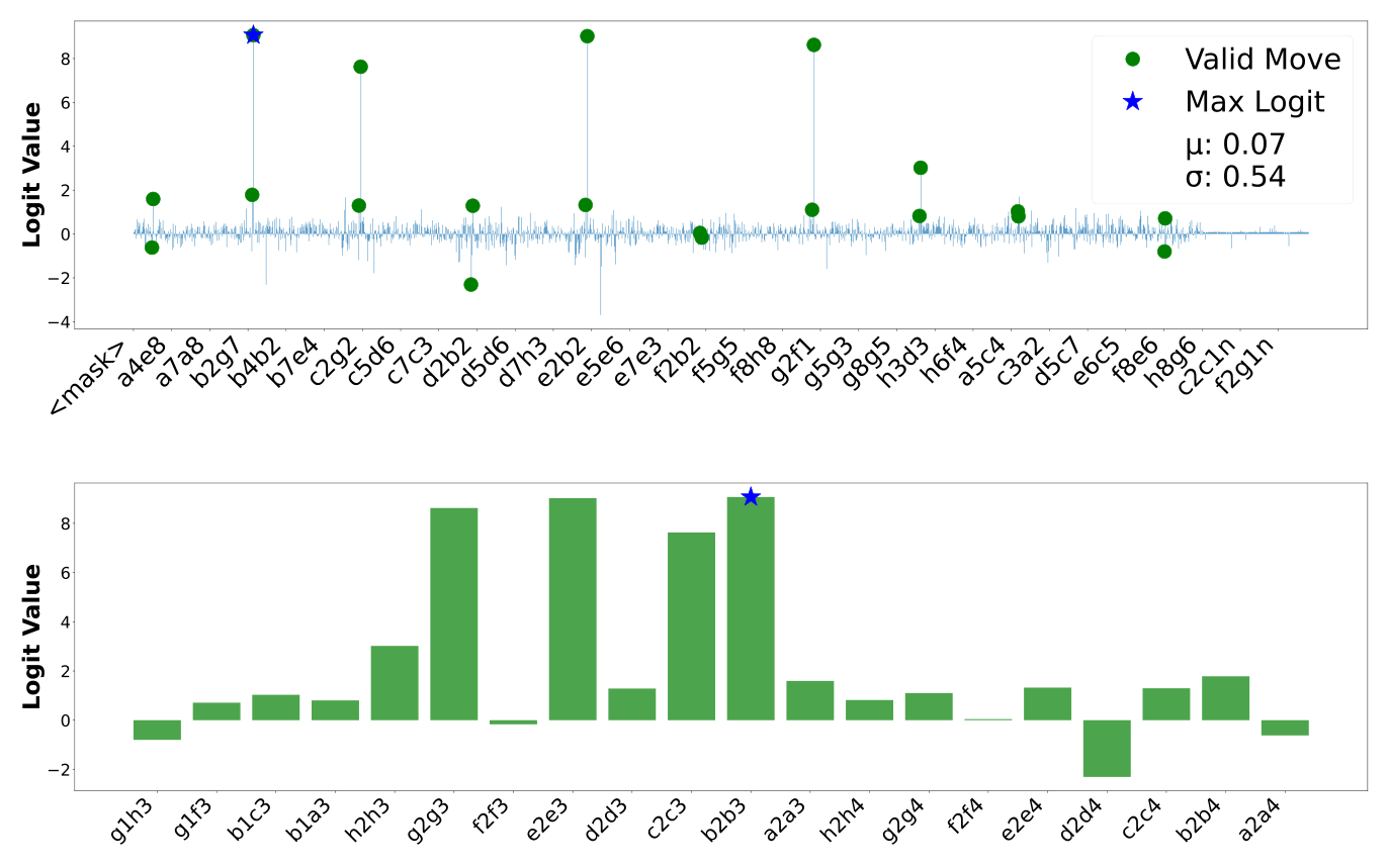
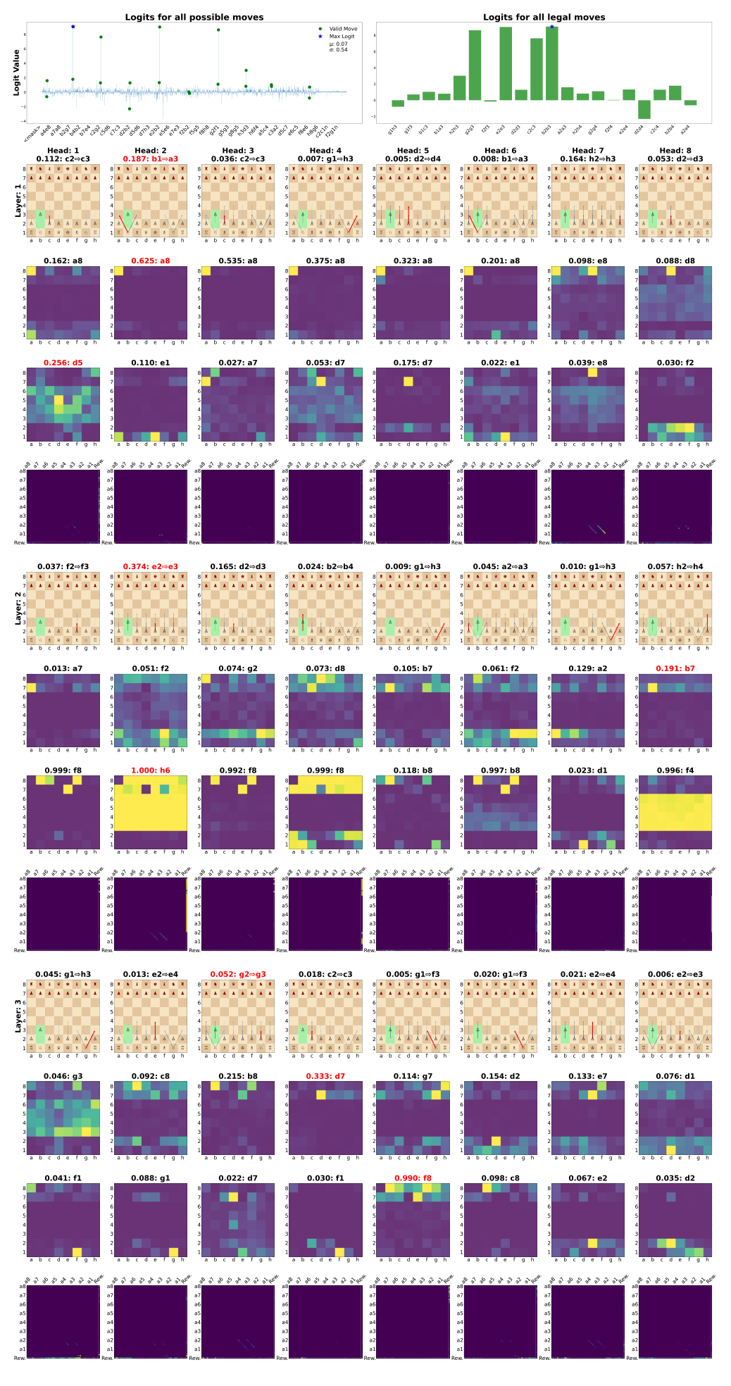
After the attention calculation, a feed forward network is applied which outputs logits. The logits represent the model’s confidence in each possible action. The logits can be visualized as a bar chart, where the x-axis represents the possible actions and the y-axis represents the confidence of the model in each action. The following image shows an example of the logits for a given board position. The first visualization shows the logits of all possible actions, with green markers for legal moves and a blue star as marker for the chosen action. The second visualization is a filtered view of the first one and just shows the logits for the legal moves. This makes the visualization easier to interpret.
As chess has many possible actions, the first visualization can get quite cluttered. The readers should focus on how many legal and illegal moves the model considers and therefore on the relative height, distribution and distance between the bars, instead of the exact values. Additionally the mean and standard deviation of the logits are shown, to provide an intuition of the model’s focus.
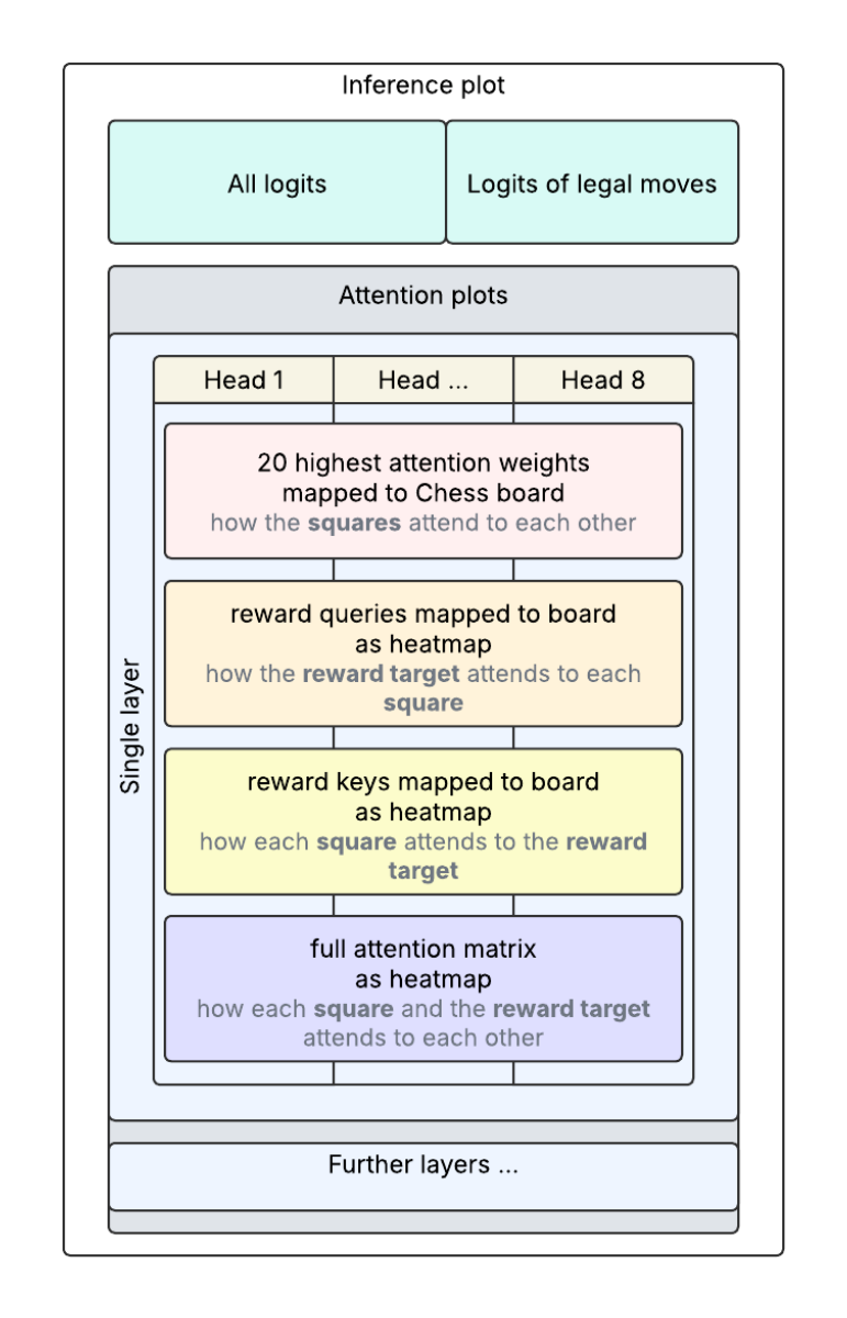
All mentioned visualizations are shown later in combination. The structure of these visualizations starts with the logits shown on top, followed by all attention heads for all or just selected layers. For each layer up to four distinct attention visualizations are presented. First, the 20 highest attention weights are visualized on the chess board. Second, the visualization shows how the reward token (query) attends to individual board squares (keys) on an 8x8 matrix representing the chess board. Third, the inverse visualization shows how each board square (query) attends to the reward token (key). Lastly, the full attention matrix is shown as heatmap, with or without masking on just legal moves. This structure is shown in the next image as well.
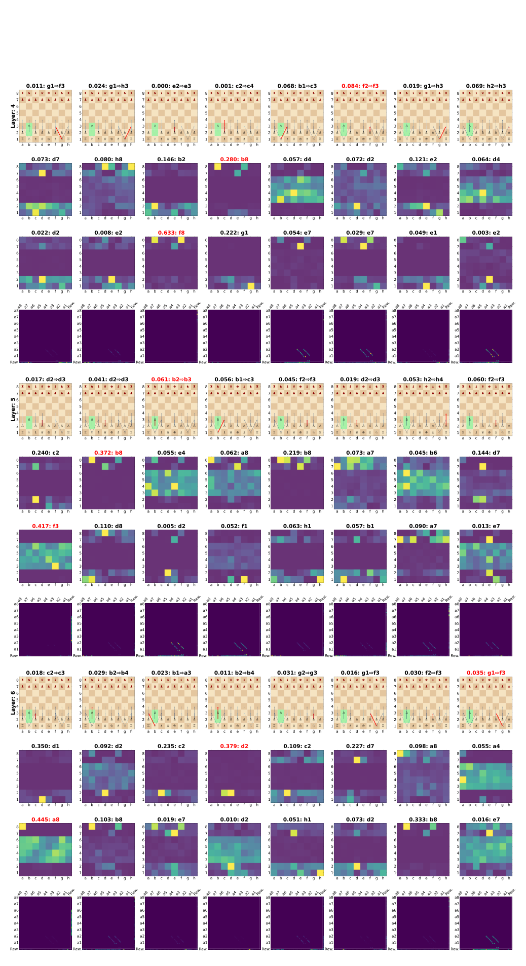
An example of such a visualization is shown below. As the visualizations get quite big with all layers shown, most of the later presented visualizations just show the first layer and last layer. The full images, including versions with all and limited layers and with and without masking on legal moves, are stored online, for the reader to explore further.13 The repository does not just hold the images for a single move as shown here, but for a full game.
In most experiments this visualization is always shown with the exact same board state, to make the visualization comparable between different models. The selected board state to display is a position from game 16 of the World Chess Championship 1985 between Karpov and Kasparov, after blacks 6th move.14 This position was chosen because, typical of the midgame, both players have numerous options, and the position is relatively balanced, with the white player holding a slight advantage of +32 centipawns. As mentioned earlier, the active player rarely has a chance to improve their position by a large margin. This is the case here as well, as the best move just keeps this advantage. The five best possible white moves are shown in the table below. Furthermore, a white piece is currently under pressure on e4 and could be captured by the black player’s knight on the next turn. The outermost left image below shows the situation, including black’s last move shown on grey squares, and the white move selected by Karpov. Further the following two half moves are shown.
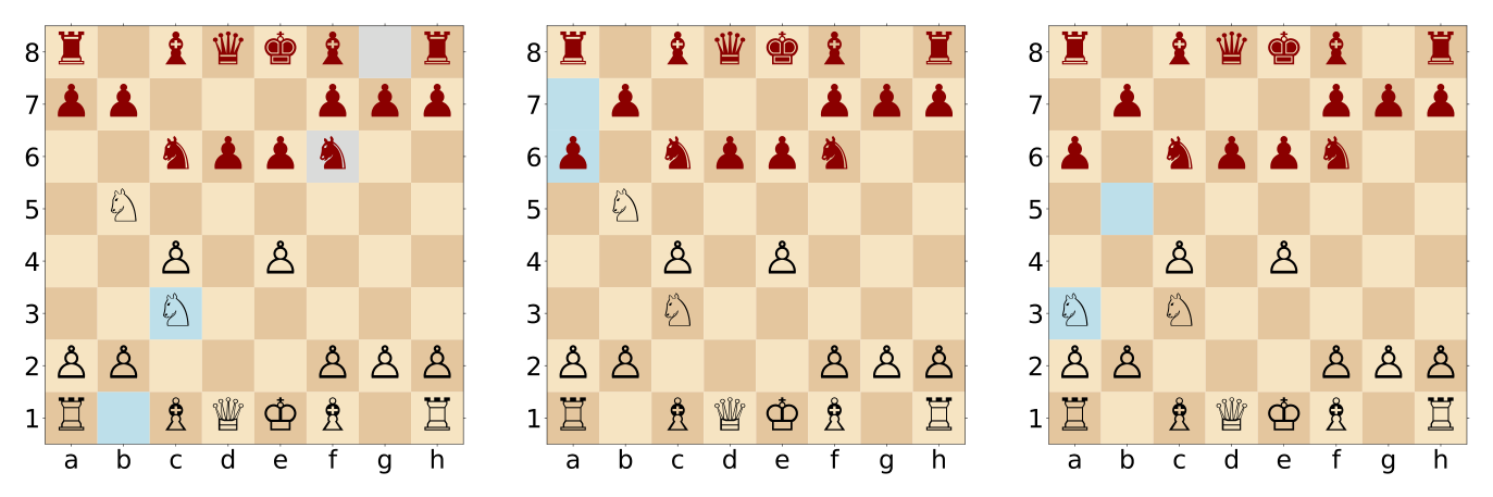
The next table shows the five best possible white moves in this position, with the evaluation after each move.
| Move | Evaluation after the move in centipawns |
|---|---|
| N5c3 - Knight from B5 to C3 | +32 |
| N1c3 - Knight from B1 to C3 | +25 |
| Bd3 - Bishop from F1 to D3 | +21 |
| Bg5 - Bishop from C1 to G5 | +6 |
| Nd2 - Knight from B1 to D2 | -25 |
Best possible white moves - source: own depiction
According to the engine’s evaluation Karpov played the second best move with N1c3.
Codebase
As mentioned, the code for the experiments is based on the Chess-Transformer project. Therefore, a high-level explanation of the initial code is provided first, followed by a discussion of the additions implemented for the conducted experiments.
The Chess-Transformer project is written in Python and uses the PyTorch library for the neural network components. The code is structured in a modular way, with separate files for components such as data preprocessing, different models, and training procedures. The main components and how they interact with each other are shown in the visualization below. The models are loaded via configuration files. As the newly designed models are based on the Transformer architecture and optimize for just the next action given the state input, just the encoder-only configuration is relevant here.
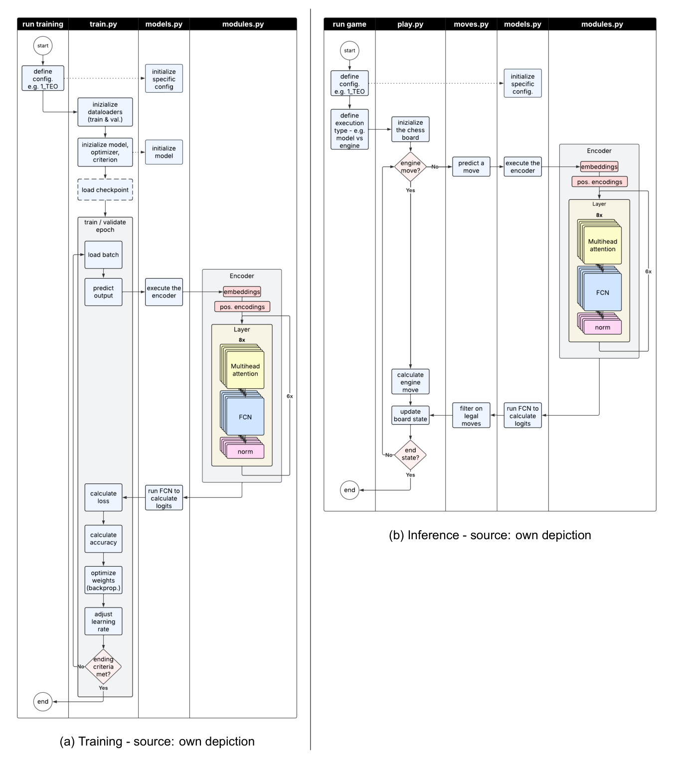
The next visualization shows the encoder model in detail and how the inputs are transformed until the model predicts the next action. The implementation of the attention mechanism closely resembles the NanoGPT project, a minimalist implementation of the GPT architecture by Andrej Karpathy, released in December 2022.15
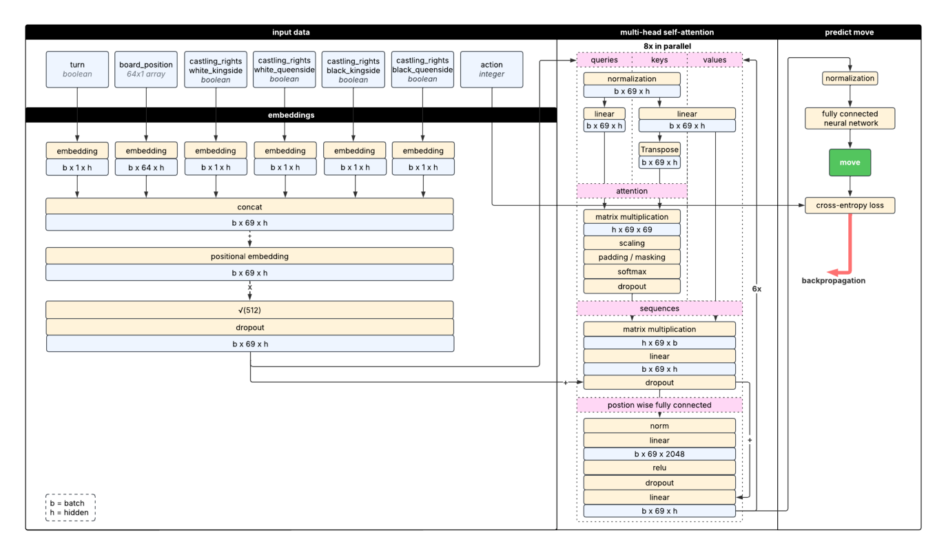
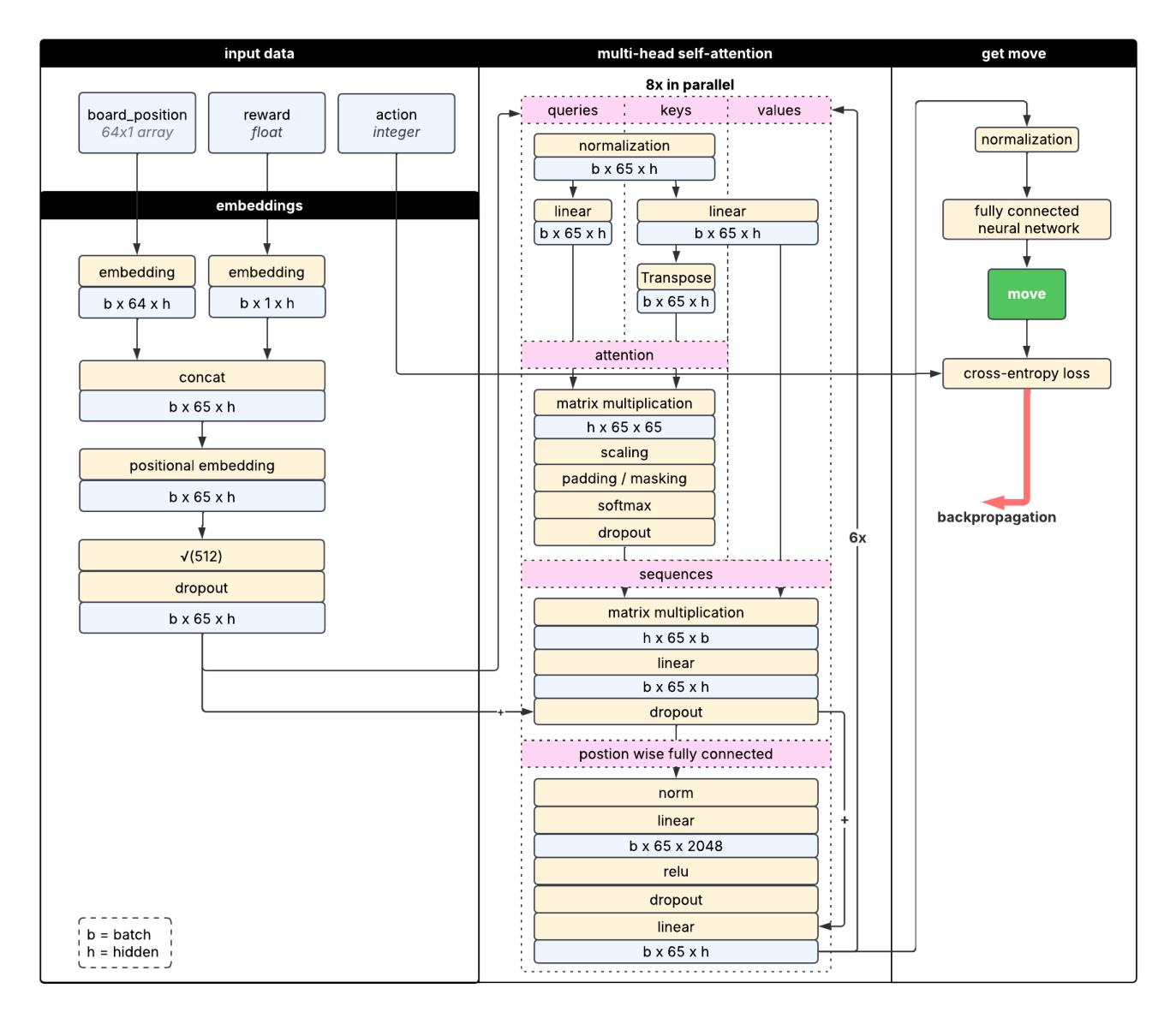
To reduce the model’s inputs for the experiments, certain features, such as castling rights, were removed. Given that the models are evaluated comparatively rather than for absolute playing strength, a possible loss in capabilities was deemed acceptable.
The following image shows the architectural change for the UDRL architecture and how the reward signal is incorporated into the model.
Switching the model to use a RTG required only an adjustment to the reward calculation, as shown in the visualization below. In this case future rewards are summed up to create the RTG for each time step.
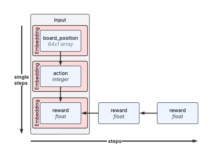
The DT architecture adds a past trajectory of states, actions, rewards and the timestep of these as input to the model. The adjustment in the structure of the input data is shown in the visualization below.
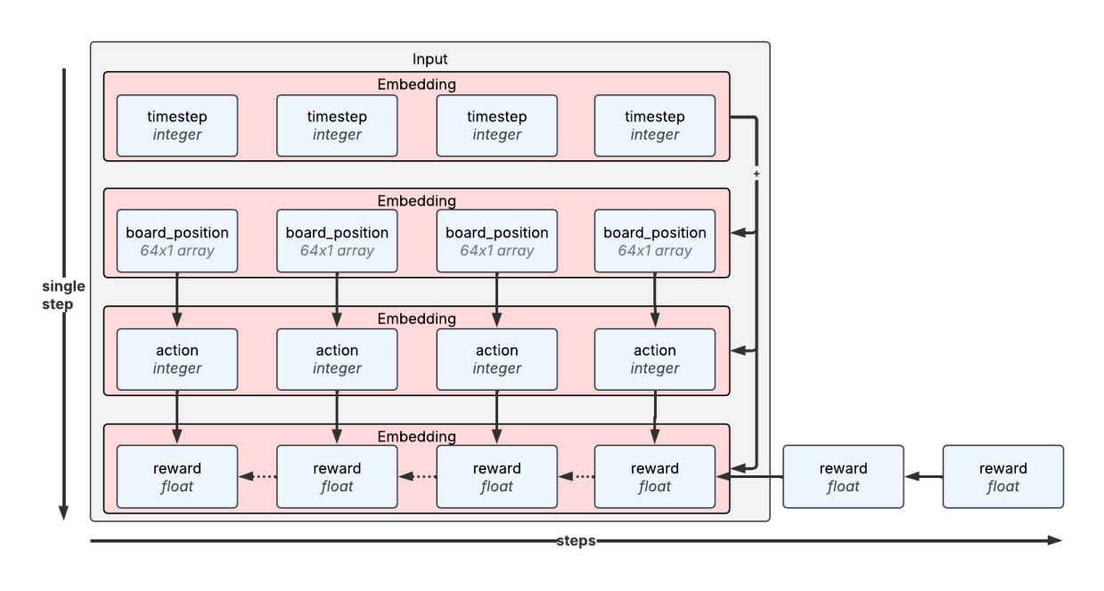
Beyond this input shaping, the DT architecture remains very similar to the UDRL architecture, with the key difference being the addition of causal masking in the attention layer to prevent the model from attending to future time steps in the trajectory.
Data preprocessing
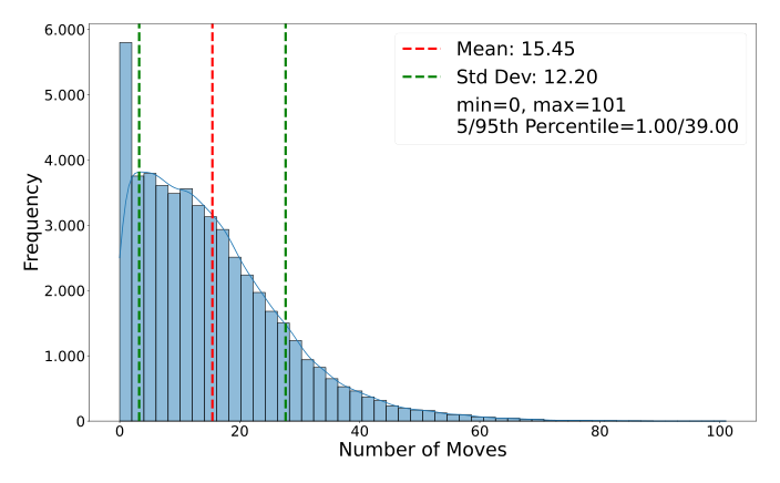
The training data provided by the Chess-Transformer project was not used due to already being filtered on playing strength. Therefore, new game data was sourced from the Lichess platform.16 Lichess provides the games played on the platform to the public under the Open Database License.17 The data is provided in PGN format, which is a standard format for storing chess games. The data includes games from players with various skill levels using the platform. For the experiment, the data from July 2025 was used as a starting point, which offered 93.092.772 games. Out of this the first 500.000 games were selected for further processing.18 The games had a length between 0 and 110 moves, resulting in 16.481.018 moves summed up over all games.19 Not all of these moves were visited during a training epoch, the reason for this gets explained in detail later. The distribution of game lengths is shown in the following visualization.
The selected 500.000 games were then processed via a custom Python script, which used the “python-chess” library20 to parse the PGN files and extract the relevant information. Several relevant data points were stored in the final training dataset. Compare the earlier mentioned tokenization process as well (compare input representation).
The board position is represented as a 1D array of 64 elements, with the entries being numbers from 2-13 for the different pieces, while the number 0 represents an empty square and the number 1 indicates a possible en-passant square.21 For example, the number 2 represents the black pawn. If the number 2 is stored at position 8 in the array (indexed at 0), this corresponds to the pawn on the second rank and first file (a7), which is the starting position of the outermost left black pawn. The 1D array representation can be easily transformed back to a 2D board representation, by reshaping the array to an 8x8 matrix.
The actions executed by a player have been stored as integers mapped to a lookup table of possible legal moves. An example for that would be the move “e2e4”, which would be mapped to the integer 758. The list of legal moves was taken from the Chess-Transformer project and has a length of 1968 moves, plus a padding token at 0, which is to be ignored during training. This representation makes it easy to use the actions as targets for the classification task during training.
Further Lichess added an evaluation of each move to the PGN file for certain games. To reduce the computational costs, only games which provided this information were used. Additionally, the material difference was calculated after each move and stored, as explained earlier.
Next the legal moves at the given position are calculated, by querying the initialized Python chess library for this information and saving it as a list of legal moves. This list was later transformed to a 64x64 matrix of boolean values to then mask the illegal moves.
All preprocessing focused exclusively on the white player’s moves, as the experiments are conducted solely from the perspective of the white player. This was done as the focus of the experiments is not on the differences between the white and black player. This reduced the amount of data and computational costs for preprocessing, training and inference for the experiments.
The table below shows an example of the preprocessed data, with the black move shown for context. The reward is shown as calculated by the evaluation engine and by the material difference approach. Further the number of legal moves is shown and a short explanation of the move is given.
| Turn | 1 | 2 | 3 |
|---|---|---|---|
| Player | White | Black | White |
| Board Position | [5, 7, … 6, 4] | [5, 7, … 6, 4] | [5, 7, … 6, 4] |
| Action | e2e4 | d7d5 | e4d5 |
| Reward difference (Evaluation-based) | +23 | – | +54 |
| Reward difference (Material-based) | 0 | – | +1 |
| Legal Moves | 20 moves available | – | 20 moves available |
| Explanation | Opening move | – | Pawn takes pawn |
Training data example - source: own depiction
The data was stored in the Apache Arrow file format, a “universal columnar format […] for fast data interchange and in-memory analytics”, to be then read during training.22 One game was stored as one row in the file, which had the advantage that sequence modeling of the data was easy to be applied during data loading. The disadvantage of storing one game per row, as opposed to one move per row, is that to sample multiple or all moves within a single game, the row must be accessed multiple times. To make this possible, a training loop was implemented to visit each game multiple times per epoch, controlled by a configuration parameter (set to 20).23 This did result in 10 million training samples per epoch (500.000 games × 20 visits), with 10% of these games used for validation. During training the data was loaded as a PyTorch dataset, which made use of the PyTorch data loader for efficient batching, shuffling and multiprocessing during training.
Reward distribution
The experiments used one of the mentioned two types of rewards, either evaluation difference-based by a chess engine or the calculated material difference value. This reward was either an instantaneous value after a single move or included future states as RTG, which is the cumulative sum of the rewards for the next actions. These four possible setups are listed below, to show the possible combinations clearly.
- Reward based on evaluation difference
- Reward based on material difference
- RTG based on evaluation difference
- RTG based on material difference
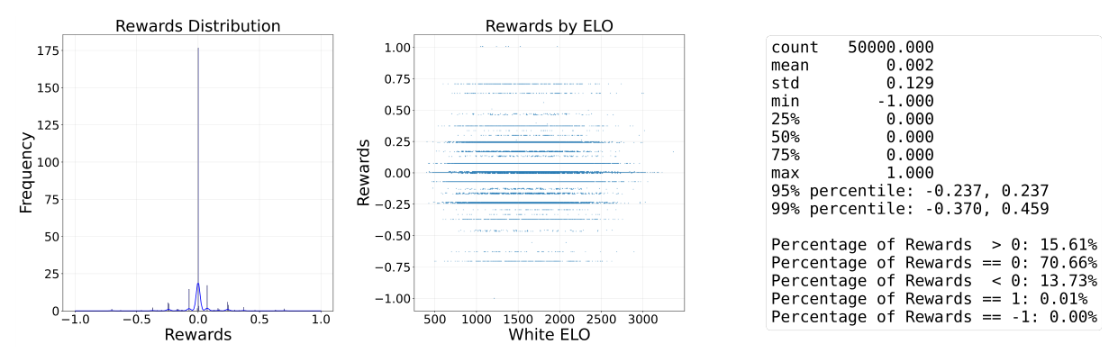
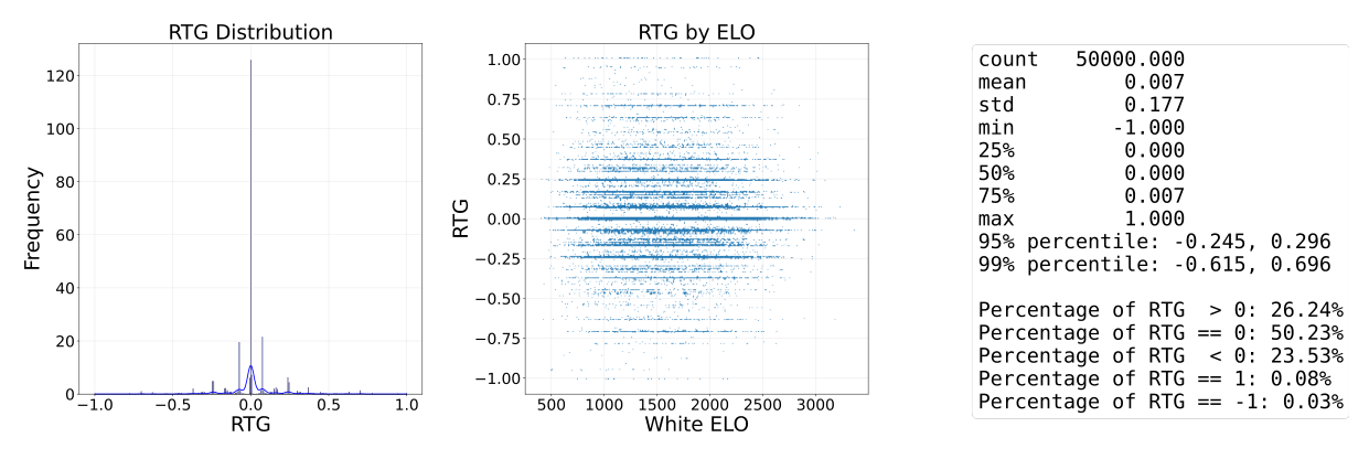
As these types of rewards are used as input and steering signal for the models, their distribution is analyzed here in detail. This is done on a sample of 50.000 moves, which are part of the training dataset. The mean, standard deviation and further relevant values are shown on the image. First, the evaluation based reward type is shown. The RTG is always shown with a trajectory length of 3 steps.
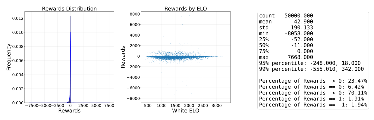
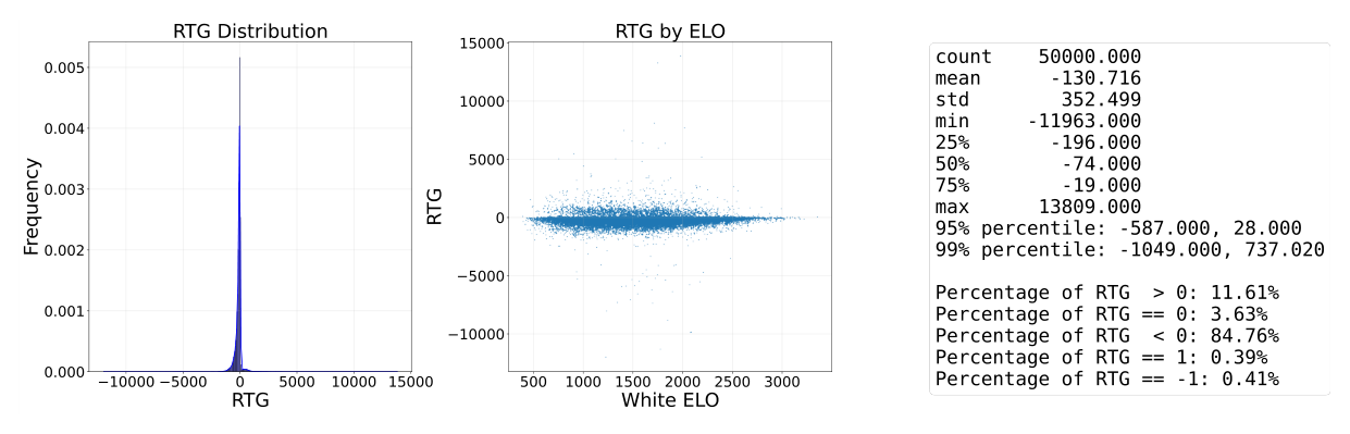
It is visible that the evaluation difference-based reward type is skewed to negative values (compare scaled image as well below). As previously mentioned, it is harder to improve a position than to worsen it with suboptimal play. The evaluation by the chess engine is forward looking and assumes perfect (super-human) play by both sides from the point of the evaluation onwards. Therefore, it is more likely that a human player makes a suboptimal move, which worsens their position, instead of improving it. In a game this happens on both sides and therefore evens out if both players have the similar skill level. As the reward is calculated just for the white player’s moves, this results in a skew to negative reward values.
The next visualizations show the distributions for the material difference-based reward types. Here the distribution is more balanced between positive and negative rewards, as the calculation is based on the combined effect of the white and black player moves on material count. Further the distribution is discrete, as material count only changes in discrete steps when pieces are captured.24
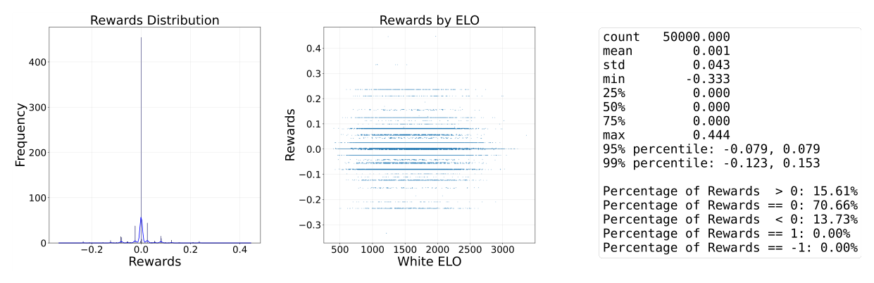
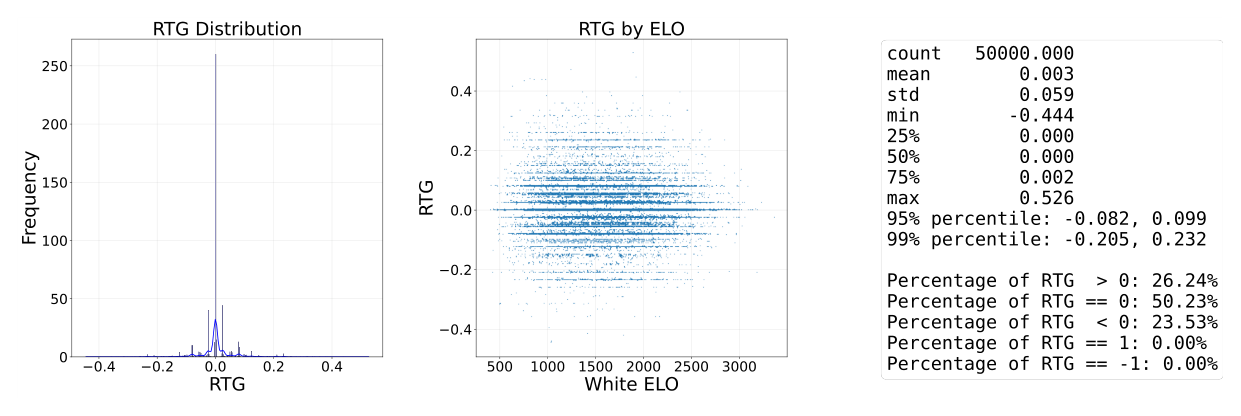
It is important to note that in both cases a reward value of 0 is the most common outcome, as many moves do not change the evaluation or material count. Overall inference with a reward target of 0 should lead to reasonable play, as the model learns to avoid moves that would substantially worsen the position.
To make the input values numerically better for a neural network both types of rewards were scaled. For the plain reward the values have been adjusted by dividing the values by a value of 500, a normalization constant determined through analysis of the distribution, and then clipped to result in values between -1 and 1.25 The RTG was scaled to a range between -1 and 1 by dividing the values by a value of 1.000 and then clipped. The resulting distribution is shown below.
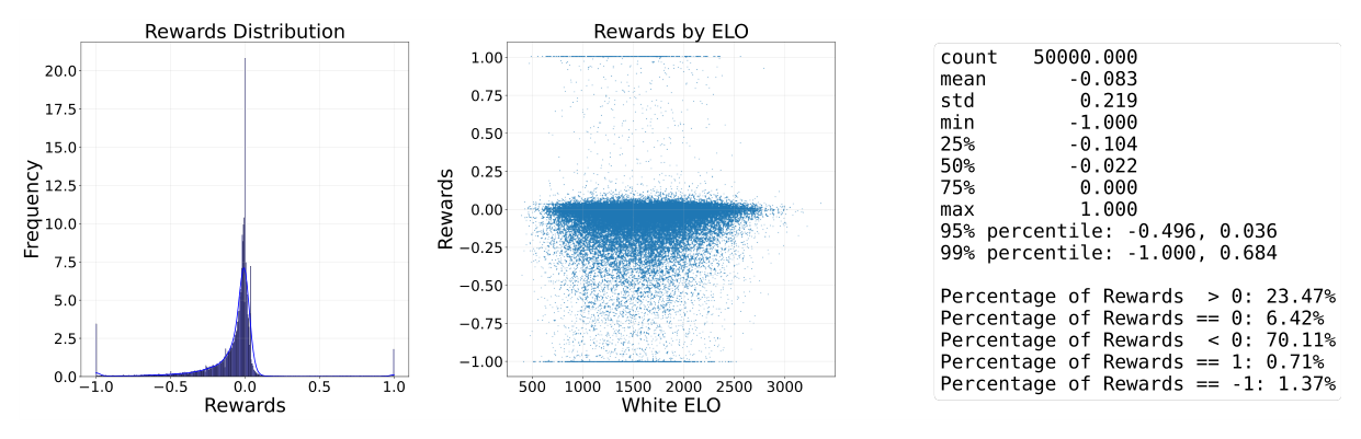
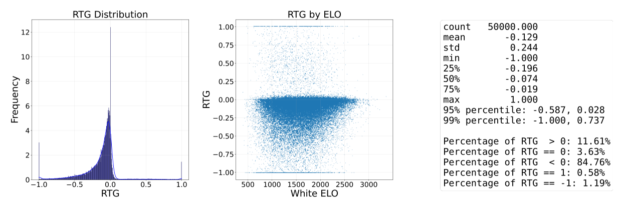
The scaled evaluation difference-based reward distribution shows that positive values are rather rare in the sample. This is again due to the fact that improving a position is harder than worsening it with suboptimal play. Therefore, the model will see more negative reward values during training. Potential implications will be analyzed during the experiments.
The next visualizations show the scaled distributions for the material difference-based reward types. For scaling a constant of 3 was used to multiply the values and then clipped to a range between -1 and 1.
The material difference-based reward and RTG distributions have a lower variance compared to the evaluation difference-based distributions. This is because the material difference only changes in discrete steps when pieces are captured, while the evaluation can change more fluidly and in a wider range for each move. Overall the numerical values of both reward types are in itself not as relevant, but need to provide a consistent signal to the model to learn from. Further the reward target during inference needs to align with the reward distribution seen during training.
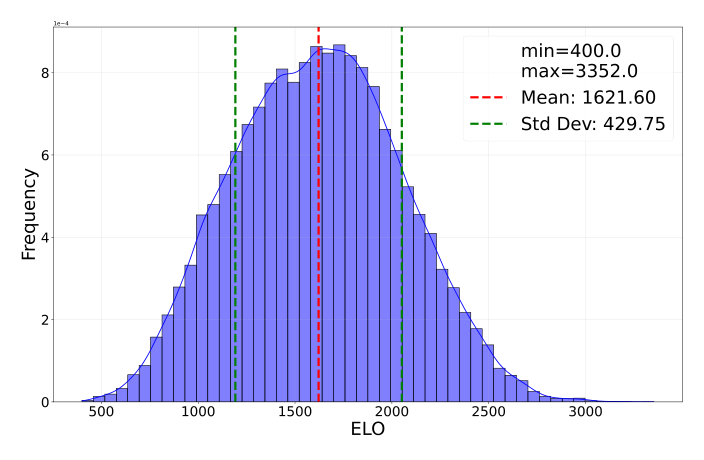
Below the distribution of the players Elo in the training dataset is shown. The mean Elo is 1.622, with a standard deviation of 430. Games from players with Elo of exactly 1.500 have been excluded in the training and evaluation dataset, as this is the default starting value for new Lichess players, which caused a significant peak in the distribution. This would still leave games from players which have not found a final first rating yet, as that would take multiple games with possible larger changes in their Elo. As this error is less relevant and more complicated to identify it is accepted. The adjustment is visible as a small dip in the image at 1.500 Elo.
Next the reward distribution is analyzed with regard to the player’s Elo. The Elo bins were defined as 500-1.250, 1.250-2.000 and 2.000-2.750. The distribution of the reward per Elo bin is shown below. Testing the distribution being normal distributed was done via the Shapiro-Wilk (SW) test and testing the bins for equal distribution was done via the Kolmogorov-Smirnov (KS) test. The results, the according test statistic and the p-value are shown in the tables below.
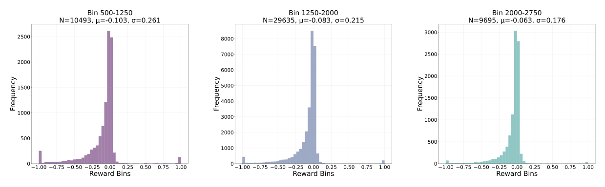
The test for being normal distributed rejected the null hypothesis. The test for equal distribution failed to reject the null hypothesis, even as the visualization shows less large negative values for the highest Elo bin. This is expected, as higher Elo players tend to make fewer critical mistakes. The values are shown in the tables below.
| Elo Bin | Count | Mean | Std | SW | p-value | |
|---|---|---|---|---|---|---|
| 500-1.250 | 10.493 | 0,002 | 0,141 | 0,196 | <0,001 | Reject null hypothesis of normality. |
| 1.250-2.000 | 29.638 | 0,003 | 0,127 | 0,184 | <0,001 | Reject null hypothesis of normality. |
| 2.000-2.750 | 9.695 | 0,002 | 0,122 | 0,176 | <0,001 | Reject null hypothesis of normality. |
evaluation difference-based reward - statistical analysis of standard distribution per Elo bin - source: own depiction
| Elo Bins | KS | p-value | |
|---|---|---|---|
| 500-1.250 vs 1.250-2.000 | 0,160 | 0,494 | Null hypothesis of similar distributions can not be rejected. |
| 500-1.250 vs 2.000-2.750 | 0,060 | 1,000 | Null hypothesis of similar distributions can not be rejected. |
| 1.250-2.000 vs 2.000-2.750 | 0,180 | 0,350 | Null hypothesis of similar distributions can not be rejected. |
evaluation difference-based reward - statistical analysis of equal distribution per Elo bin - source: own depiction
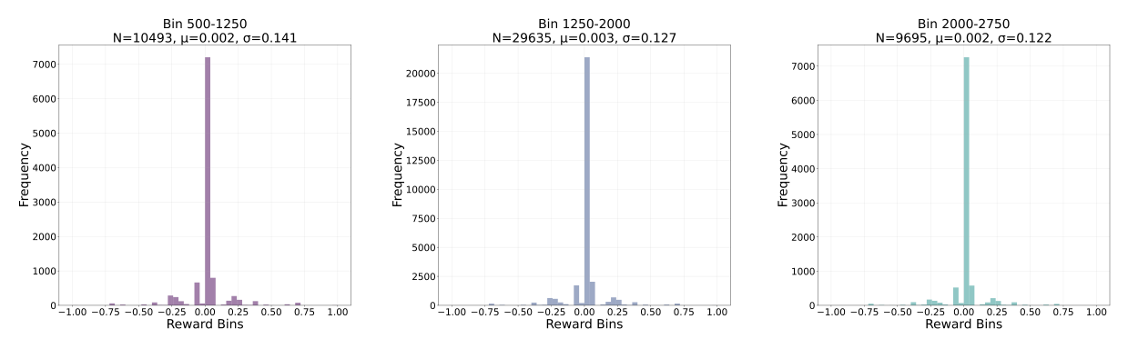
For the material difference-based reward type the test for being normal distributed was negative for all bins as well. The test for equal distribution of the null hypothesis could not be declined for the first two comparisons, but for the comparison for the 1.250-2.000 and 2.000-2.750 bins.
| Elo Bin | Count | Mean | Std | SW | p-value | |
|---|---|---|---|---|---|---|
| 500-1.250 | 10.493 | 0,002 | 0,141 | 0,4242 | <0,001 | Reject null hypothesis of normality. |
| 1.250-2.000 | 29.638 | 0,003 | 0,127 | 0,3875 | <0,001 | Reject null hypothesis of normality. |
| 2.000-2.750 | 9.695 | 0,002 | 0,122 | 0,3526 | <0,001 | Reject null hypothesis of normality. |
Material difference-based reward - statistical analysis of standard distribution per Elo bin - source: own depiction
| Elo Bins | KS | p-value | |
|---|---|---|---|
| 500-1.250 vs 1.250-2.000 | 0,2200 | 0,153 | Null hypothesis of similar distributions can not be rejected. |
| 500-1.250 vs 2.000-2.750 | 0,1800 | 0,350 | Null hypothesis of similar distributions can not be rejected. |
| 1.250-2.000 vs 2.000-2.750 | 0,3200 | 0,009 | Reject null hypothesis of similar distributions. |
Material difference-based reward - statistical analysis of equal distribution per Elo bin - source: own depiction
As the players were paired by their Elo in the games the reward distribution should be similar across all Elo levels. Just minor statistical differences between the analyzed Elo bins and the reward distribution were found. This means that the reward distribution is similar for almost all player levels and indicates that the Elo model works well in chess. Therefore, the reward provides a consistent signal across different skill levels without leaking the Elo information directly to the model.
Continue with Part 3: Results - Chess-Transformer baseline and base UDRL, which covers the training metrics of all models and the results for 1_TEO, 2_UDRL-eval, 3_UDRL-material and 4_UDRL-eval-legal_input.
References
https://gitlab.com/iu-msc-ai/transformer-based-offline-reinforcement-learning-applied-to-chess/-/tree/main/chess_transformers/configs/models ↩︎
https://huggingface.co/micha-net/transformer-based-offline-reinforcement-learning-applied-to-chess ↩︎
Most of these settings can be found in the base configuration file: https://gitlab.com/iu-msc-ai/transformer-based-offline-reinforcement-learning-applied-to-chess/-/tree/main/chess_transformers/configs/models/EXP_base.py ↩︎
Bruce, Peter; Bruce, Andrew; Gedeck, Peter - Practical Statistics for Data Scientists, O’Reilly Media, 2020, p. 124-129. ↩︎
Little, Todd - The Oxford Handbook of Quantitative Methods, Volume 2: Statistical Analysis, Oxford University Press, 2013, p. 92. ↩︎
https://docs.scipy.org/doc/scipy/reference/generated/scipy.stats.fisher_exact.html ↩︎
Playing 500 games between Stockfish and one of the models took around 90 minutes, if both players had equal playing strength. ↩︎
All results are shown in a comprehensive table in the appendix of part 4, including values for the confidence intervals, based on the Wilson score interval. ↩︎
Stockfish - Frequently Asked Questions - How do Skill Level and UCI_Elo work, accessed 2025-10-24. https://official-stockfish.github.io/docs/stockfish-wiki/Stockfish-FAQ.html#how-do-skill-level-and-uci-elo-work ↩︎
The masking of illegal moves was just done for the visualization of the attention on the chess board and the shown full attention matrix, not for the plots showing the reward attention. Here the attention pattern was already comprehensible even without the filter. ↩︎
An alternative would have been to embed the whole board state into a single token. In that case it would not have been possible to show the attention on the individual board squares afterwards. ↩︎
Link to the visualizations: https://drive.google.com/drive/u/0/folders/1hdufR-XJG6hZEuTcZ9coDUh5oRrGmwcY ↩︎
The full game can be found here: https://www.chess.com/blog/ThummimS/world-chess-championship-1985-game-16-karpov-vs-kasparov ↩︎
Lichess is a “free/libre, open-source chess server powered by volunteers and donations”. Compare 26. ↩︎
Just games with stored evaluation were taken, compare below. ↩︎
Games with a very low number of moves could be due to a player deliberately forfeiting a game. ↩︎
The lookup tables used to encode the pieces and all possible actions can be found here: https://gitlab.com/iu-msc-ai/transformer-based-offline-reinforcement-learning-applied-to-chess/-/tree/main/chess_transformers/data/levels.py ↩︎
Apache Software Foundation - Apache Arrow, accessed 2025-11-24. https://arrow.apache.org/ ↩︎
When games did not have 20 white moves per game moves were visited multiple times per epoch. This seems to have no negative effect on the training, but reduces the variety of samples seen per epoch. ↩︎
The value was calculated with following centipawn values: pawn=100, knight=320, bishop=330, rook=500, queen=950. Then the difference between the white and the black player material was divided by the maximum available material on the board, which is 4.500. ↩︎
Scaling via the mean and standard deviation was experimented with as well, but did not show better results. ↩︎
Lichess - About lichess.org, accessed 2025-11-24. https://lichess.org/about ↩︎